Analysis
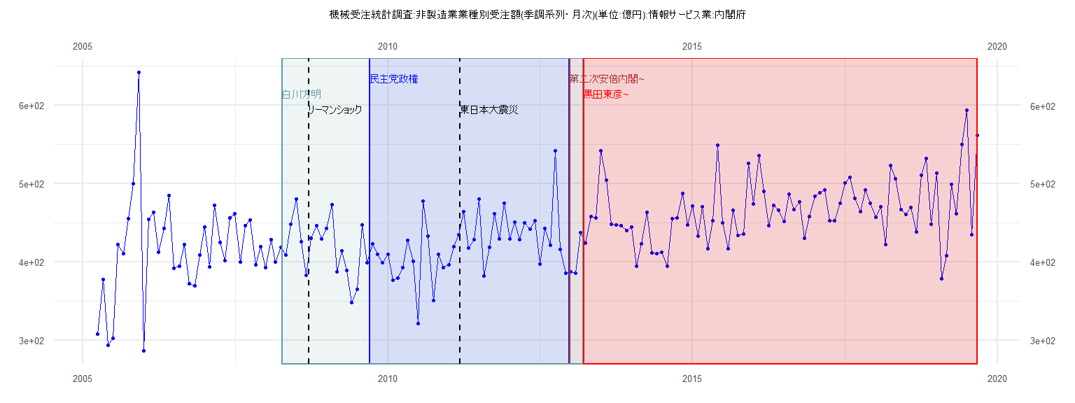
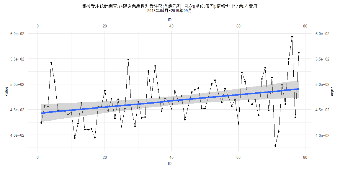
[1] "機械受注統計調査:非製造業業種別受注額(季調系列・月次)(単位:億円):情報サービス業:内閣府"
        Jan    Feb    Mar    Apr    May    Jun    Jul    Aug    Sep    Oct    Nov    Dec
2005                      307.87 377.79 293.71 302.41 421.79 410.68 455.14 499.63 641.88
2006 286.77 454.60 463.29 412.50 443.05 484.55 391.57 394.44 422.40 372.27 369.21 408.98
2007 444.37 393.23 472.10 424.59 401.36 455.87 461.31 400.18 446.51 453.69 396.70 419.14
2008 392.96 428.62 399.78 418.24 408.64 447.64 480.39 426.09 383.02 429.86 446.60 429.46
2009 442.95 473.38 387.55 414.09 389.25 348.36 364.76 447.15 398.66 423.01 409.83 398.80
2010 409.89 376.27 378.89 392.39 427.36 400.71 321.64 477.62 432.59 351.13 409.59 392.89
2011 396.56 419.10 434.94 464.37 417.42 428.75 480.60 382.24 418.19 461.62 429.58 474.83
2012 429.35 450.38 428.65 449.67 441.80 452.56 397.49 443.12 420.85 541.83 415.72 385.18
2013 387.29 385.33 437.65 423.62 457.54 456.27 542.09 504.39 448.49 447.11 446.38 440.35
2014 444.47 394.20 422.68 463.41 411.18 410.50 412.33 394.57 455.21 456.55 487.49 447.35
2015 471.57 433.21 470.22 416.36 452.32 548.91 450.13 417.23 466.11 433.66 435.57 526.17
2016 474.36 536.02 489.68 446.58 471.96 465.77 451.38 486.51 466.71 476.67 430.27 458.27
2017 484.07 488.64 492.21 452.81 452.33 474.88 500.46 507.82 481.51 464.25 491.81 474.56
2018 457.14 469.98 421.85 523.31 505.75 466.92 460.26 469.29 438.14 510.54 532.34 448.09
2019 513.45 378.53 407.68 498.57 461.22 549.73 593.31 434.30 561.96
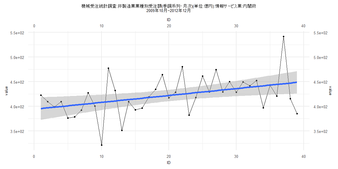
Call:
lm(formula = value ~ ID)

Residuals:
    Min      1Q  Median      3Q     Max
-86.610 -21.220  -0.108  15.522  95.804

Coefficients:
            Estimate Std. Error t value             Pr(>|t|)
(Intercept) 394.2596    11.7239  33.629 < 0.0000000000000002 ***
ID            1.3991     0.5109   2.739              0.00943 **
---
Signif. codes:  0 '***' 0.001 '**' 0.01 '*' 0.05 '.' 0.1 ' ' 1

Residual standard error: 35.91 on 37 degrees of freedom
Multiple R-squared:  0.1685,    Adjusted R-squared:  0.1461
F-statistic:   7.5 on 1 and 37 DF,  p-value: 0.009432


    Two-sample Kolmogorov-Smirnov test

data:  lm_residuals and rnorm(n = length(lm_residuals), mean = 0, sd = sd(lm_residuals))
D = 0.12821, p-value = 0.9114
alternative hypothesis: two-sided


    Durbin-Watson test

data:  value ~ ID
DW = 2.3073, p-value = 0.7886
alternative hypothesis: true autocorrelation is greater than 0


    studentized Breusch-Pagan test

data:  value ~ ID
BP = 0.78665, df = 1, p-value = 0.3751


    Box-Ljung test

data:  lm_residuals
X-squared = 1.7506, df = 1, p-value = 0.1858
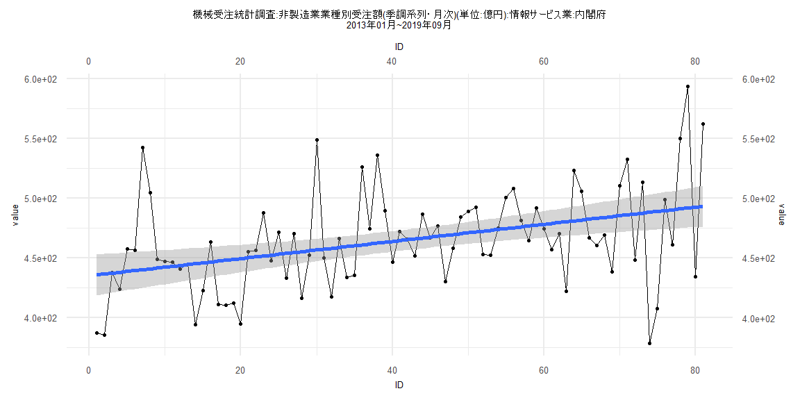
Call:
lm(formula = value ~ ID)

Residuals:
     Min       1Q   Median       3Q      Max
-109.520  -22.782    0.393   18.574  101.972

Coefficients:
            Estimate Std. Error t value             Pr(>|t|)
(Intercept) 435.1105     8.7128  49.939 < 0.0000000000000002 ***
ID            0.7154     0.1846   3.875             0.000219 ***
---
Signif. codes:  0 '***' 0.001 '**' 0.01 '*' 0.05 '.' 0.1 ' ' 1

Residual standard error: 38.85 on 79 degrees of freedom
Multiple R-squared:  0.1597,    Adjusted R-squared:  0.1491
F-statistic: 15.02 on 1 and 79 DF,  p-value: 0.0002186


    Two-sample Kolmogorov-Smirnov test

data:  lm_residuals and rnorm(n = length(lm_residuals), mean = 0, sd = sd(lm_residuals))
D = 0.1358, p-value = 0.4462
alternative hypothesis: two-sided


    Durbin-Watson test

data:  value ~ ID
DW = 1.7134, p-value = 0.07827
alternative hypothesis: true autocorrelation is greater than 0


    studentized Breusch-Pagan test

data:  value ~ ID
BP = 2.1383, df = 1, p-value = 0.1437


    Box-Ljung test

data:  lm_residuals
X-squared = 1.083, df = 1, p-value = 0.298
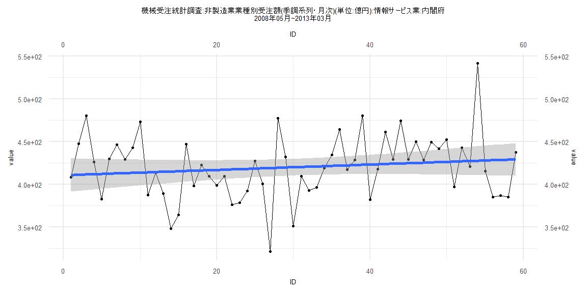
Call:
lm(formula = value ~ ID)

Residuals:
    Min      1Q  Median      3Q     Max
-97.679 -25.824  -0.509  20.446 114.015

Coefficients:
            Estimate Std. Error t value            Pr(>|t|)
(Intercept) 410.8229     9.8848  41.561 <0.0000000000000002 ***
ID            0.3147     0.2865   1.098               0.277
---
Signif. codes:  0 '***' 0.001 '**' 0.01 '*' 0.05 '.' 0.1 ' ' 1

Residual standard error: 37.48 on 57 degrees of freedom
Multiple R-squared:  0.02072,   Adjusted R-squared:  0.003539
F-statistic: 1.206 on 1 and 57 DF,  p-value: 0.2767


    Two-sample Kolmogorov-Smirnov test

data:  lm_residuals and rnorm(n = length(lm_residuals), mean = 0, sd = sd(lm_residuals))
D = 0.10169, p-value = 0.9239
alternative hypothesis: two-sided


    Durbin-Watson test

data:  value ~ ID
DW = 1.8014, p-value = 0.1825
alternative hypothesis: true autocorrelation is greater than 0


    studentized Breusch-Pagan test

data:  value ~ ID
BP = 0.12457, df = 1, p-value = 0.7241


    Box-Ljung test

data:  lm_residuals
X-squared = 0.60608, df = 1, p-value = 0.4363
Call:
lm(formula = value ~ ID)

Residuals:
     Min       1Q   Median       3Q      Max
-107.549  -21.394   -0.915   16.818  104.169

Coefficients:
            Estimate Std. Error t value             Pr(>|t|)
(Intercept) 442.5992     8.8433  50.049 < 0.0000000000000002 ***
ID            0.6124     0.1945   3.149              0.00235 **
---
Signif. codes:  0 '***' 0.001 '**' 0.01 '*' 0.05 '.' 0.1 ' ' 1

Residual standard error: 38.68 on 76 degrees of freedom
Multiple R-squared:  0.1154,    Adjusted R-squared:  0.1037
F-statistic: 9.913 on 1 and 76 DF,  p-value: 0.002345


    Two-sample Kolmogorov-Smirnov test

data:  lm_residuals and rnorm(n = length(lm_residuals), mean = 0, sd = sd(lm_residuals))
D = 0.14103, p-value = 0.4221
alternative hypothesis: two-sided


    Durbin-Watson test

data:  value ~ ID
DW = 1.7714, p-value = 0.1283
alternative hypothesis: true autocorrelation is greater than 0


    studentized Breusch-Pagan test

data:  value ~ ID
BP = 2.8054, df = 1, p-value = 0.09395


    Box-Ljung test

data:  lm_residuals
X-squared = 0.65745, df = 1, p-value = 0.4175