Analysis
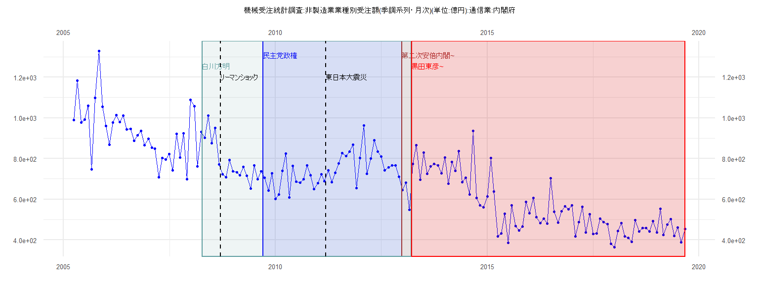
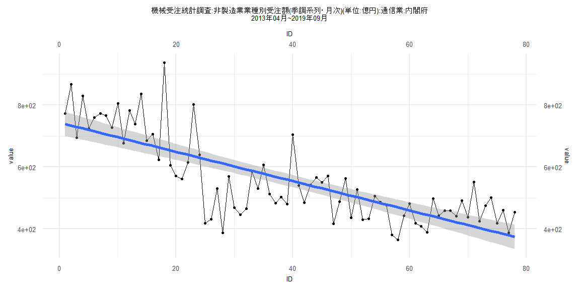
[1] "機械受注統計調査:非製造業業種別受注額(季調系列・月次)(単位:億円):通信業:内閣府"
         Jan     Feb     Mar     Apr     May     Jun     Jul     Aug     Sep     Oct     Nov     Dec
2005                          988.60 1183.32  977.90  991.34 1059.05  745.73 1099.21 1328.42 1053.74
2006  961.17  868.10  976.75 1014.00  979.35 1011.06  943.29  944.72  886.65  913.54  935.95  865.43
2007  897.14  852.85  848.23  707.88  802.33  796.37  822.10  741.43  920.34  805.43  924.48  699.55
2008 1087.44 1057.61  761.15  931.20  901.77 1010.89  876.41  950.57  772.09  722.19  707.06  792.75
2009  737.47  731.95  717.91  758.59  715.78  652.51  765.26  697.34  736.63  705.95  643.50  726.90
2010  601.84  623.02  739.82  823.78  609.57  764.14  686.62  681.19  699.50  767.09  716.87  650.91
2011  678.21  722.08  688.57  741.14  683.94  729.94  775.09  827.62  812.74  833.83  869.08  653.70
2012  801.71  962.91  726.09  800.73  888.73  834.70  808.96  740.94  756.33  765.27  767.37  711.04
2013  645.51  680.84  549.01  773.20  866.86  695.48  829.73  724.05  760.51  772.55  765.72  727.37
2014  805.90  676.52  783.42  739.42  836.13  685.08  705.68  623.66  937.10  605.30  570.84  561.10
2015  614.51  801.90  638.90  417.91  431.59  529.84  386.68  569.09  468.77  446.20  466.25  585.79
2016  530.56  606.81  512.02  483.84  503.67  480.76  704.21  539.67  485.53  541.37  565.59  549.76
2017  570.71  416.88  488.16  563.46  436.49  527.40  430.28  432.91  505.49  487.05  477.66  380.22
2018  365.05  442.77  481.77  417.63  408.90  389.85  498.05  442.23  459.56  458.70  440.91  491.78
2019  437.40  551.88  425.38  475.07  501.81  418.58  460.43  388.03  453.77
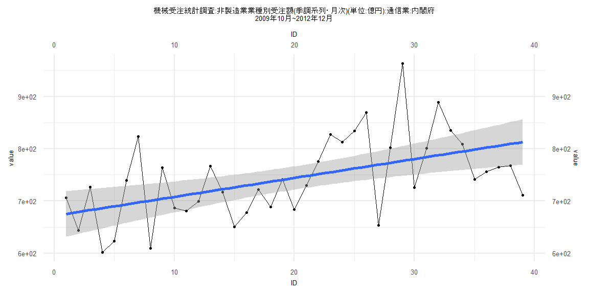
Call:
lm(formula = value ~ ID)

Residuals:
    Min      1Q  Median      3Q     Max
-115.78  -49.89  -11.20   45.32  186.20

Coefficients:
            Estimate Std. Error t value             Pr(>|t|)
(Intercept) 671.7495    22.3047  30.117 < 0.0000000000000002 ***
ID            3.6195     0.9719   3.724             0.000651 ***
---
Signif. codes:  0 '***' 0.001 '**' 0.01 '*' 0.05 '.' 0.1 ' ' 1

Residual standard error: 68.31 on 37 degrees of freedom
Multiple R-squared:  0.2726,    Adjusted R-squared:  0.253
F-statistic: 13.87 on 1 and 37 DF,  p-value: 0.000651


    Two-sample Kolmogorov-Smirnov test

data:  lm_residuals and rnorm(n = length(lm_residuals), mean = 0, sd = sd(lm_residuals))
D = 0.17949, p-value = 0.5622
alternative hypothesis: two-sided


    Durbin-Watson test

data:  value ~ ID
DW = 1.9097, p-value = 0.3238
alternative hypothesis: true autocorrelation is greater than 0


    studentized Breusch-Pagan test

data:  value ~ ID
BP = 0.61803, df = 1, p-value = 0.4318


    Box-Ljung test

data:  lm_residuals
X-squared = 0.0064651, df = 1, p-value = 0.9359
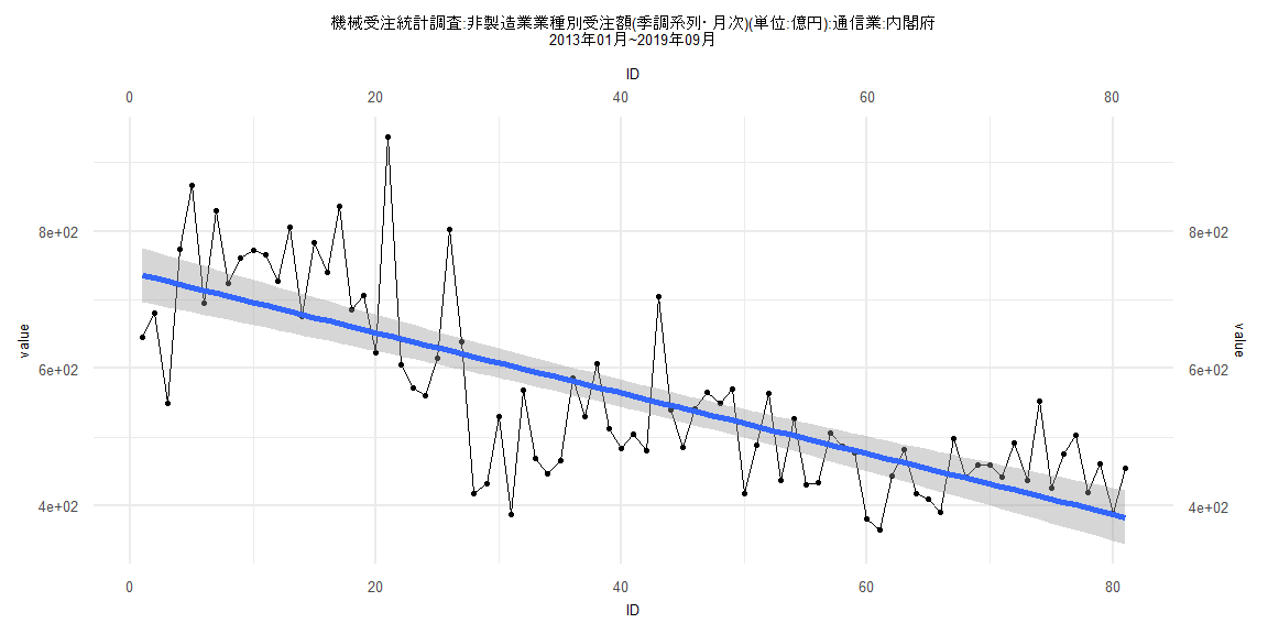
Call:
lm(formula = value ~ ID)

Residuals:
     Min       1Q   Median       3Q      Max
-216.766  -56.201    4.047   50.733  289.572

Coefficients:
            Estimate Std. Error t value            Pr(>|t|)
(Intercept) 740.1000    20.0372   36.94 <0.0000000000000002 ***
ID           -4.4082     0.4245  -10.38 <0.0000000000000002 ***
---
Signif. codes:  0 '***' 0.001 '**' 0.01 '*' 0.05 '.' 0.1 ' ' 1

Residual standard error: 89.33 on 79 degrees of freedom
Multiple R-squared:  0.5771,    Adjusted R-squared:  0.5718
F-statistic: 107.8 on 1 and 79 DF,  p-value: < 0.00000000000000022


    Two-sample Kolmogorov-Smirnov test

data:  lm_residuals and rnorm(n = length(lm_residuals), mean = 0, sd = sd(lm_residuals))
D = 0.11111, p-value = 0.7027
alternative hypothesis: two-sided


    Durbin-Watson test

data:  value ~ ID
DW = 1.4239, p-value = 0.002759
alternative hypothesis: true autocorrelation is greater than 0


    studentized Breusch-Pagan test

data:  value ~ ID
BP = 5.6833, df = 1, p-value = 0.01713


    Box-Ljung test

data:  lm_residuals
X-squared = 6.4772, df = 1, p-value = 0.01093
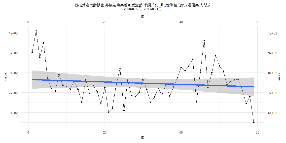
Call:
lm(formula = value ~ ID)

Residuals:
    Min      1Q  Median      3Q     Max
-181.27  -55.95  -13.32   48.70  245.38

Coefficients:
            Estimate Std. Error t value            Pr(>|t|)
(Intercept) 766.7446    23.5822  32.514 <0.0000000000000002 ***
ID           -0.6181     0.6836  -0.904                0.37
---
Signif. codes:  0 '***' 0.001 '**' 0.01 '*' 0.05 '.' 0.1 ' ' 1

Residual standard error: 89.42 on 57 degrees of freedom
Multiple R-squared:  0.01414,   Adjusted R-squared:  -0.003158
F-statistic: 0.8174 on 1 and 57 DF,  p-value: 0.3697


    Two-sample Kolmogorov-Smirnov test

data:  lm_residuals and rnorm(n = length(lm_residuals), mean = 0, sd = sd(lm_residuals))
D = 0.11864, p-value = 0.8052
alternative hypothesis: two-sided


    Durbin-Watson test

data:  value ~ ID
DW = 1.0088, p-value = 0.00001101
alternative hypothesis: true autocorrelation is greater than 0


    studentized Breusch-Pagan test

data:  value ~ ID
BP = 0.37727, df = 1, p-value = 0.5391


    Box-Ljung test

data:  lm_residuals
X-squared = 11.98, df = 1, p-value = 0.0005378
Call:
lm(formula = value ~ ID)

Residuals:
    Min      1Q  Median      3Q     Max
-224.57  -58.55    7.36   45.02  278.52

Coefficients:
            Estimate Std. Error t value            Pr(>|t|)
(Intercept) 743.7570    20.0210   37.15 <0.0000000000000002 ***
ID           -4.7322     0.4403  -10.75 <0.0000000000000002 ***
---
Signif. codes:  0 '***' 0.001 '**' 0.01 '*' 0.05 '.' 0.1 ' ' 1

Residual standard error: 87.56 on 76 degrees of freedom
Multiple R-squared:  0.6031,    Adjusted R-squared:  0.5979
F-statistic: 115.5 on 1 and 76 DF,  p-value: < 0.00000000000000022


    Two-sample Kolmogorov-Smirnov test

data:  lm_residuals and rnorm(n = length(lm_residuals), mean = 0, sd = sd(lm_residuals))
D = 0.10256, p-value = 0.81
alternative hypothesis: two-sided


    Durbin-Watson test

data:  value ~ ID
DW = 1.4204, p-value = 0.003027
alternative hypothesis: true autocorrelation is greater than 0


    studentized Breusch-Pagan test

data:  value ~ ID
BP = 3.5411, df = 1, p-value = 0.05986


    Box-Ljung test

data:  lm_residuals
X-squared = 6.5095, df = 1, p-value = 0.01073