Analysis
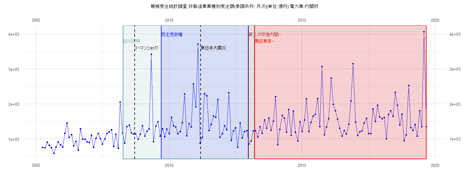
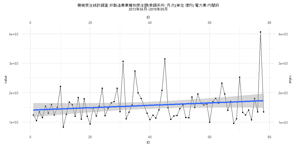
[1] "機械受注統計調査:非製造業業種別受注額(季調系列・月次)(単位:億円):電力業:内閣府"
         Jan     Feb     Mar     Apr     May     Jun     Jul     Aug     Sep     Oct     Nov     Dec
2005                          757.43  745.30  901.02  816.27  748.95  594.16  764.87  912.13  829.81
2006  766.40 1157.96 1450.60 1045.64 1125.26  802.23  926.80  680.46 1289.33  987.60  987.80  911.07
2007  895.27 1108.19  759.79 1014.12 1160.49 1006.19  853.27  999.98 1160.42 1205.18 1258.65  780.89
2008 1128.42  731.95 2050.06 1156.64  877.81 1348.51 1397.44 1174.69 1140.53 1141.10  990.98 1134.92
2009 1379.73 1081.16 1215.00 1275.78 3423.55  924.88 1370.18 1491.11 1083.27 1285.46 1061.11 1283.14
2010 1150.94 1618.33 1374.00 1344.09 1147.47 1209.48 1460.84 2287.76 1088.82 1439.45 1345.20 2568.79
2011 1918.09 3705.98  880.34 1042.90 2294.58 2232.40 1240.63 1414.03 1656.75 1617.92 2124.01 1041.94
2012 1151.83 1372.55 1265.64 2318.53  958.46 1230.96 1316.91  765.74 1451.61 1026.58 1209.56 1233.18
2013  848.11  942.52 1226.73 1240.37 1049.97 1350.40 1159.53 1543.99 1306.25 1597.86 1242.75 1503.98
2014 2209.20  832.58 1267.44 1677.18 1590.82 1195.29 1838.41 1102.06 1795.45 1194.74  937.11 1489.30
2015 1206.52 1541.50 2147.58 1213.04 1469.93 1649.97 1696.26 2156.03 1352.37 3070.20 1115.05 1343.25
2016 1580.17 2738.27 1990.70 1800.43 1564.36 1307.49 1082.51 1237.27 1136.69 1418.55 2085.02 3146.16
2017 1484.04 1097.58 1205.10 1227.20 1452.09 1585.30 1151.62 1148.57 1854.06 1494.99 1962.81 1633.07
2018 1579.29 1609.00  998.52 1696.46 1807.08 1645.25 2325.95 1962.04 1396.89 1704.44  952.45 1111.46
2019 2524.71 1326.51 1246.65 1409.77 1078.11 1806.08 1349.72 4065.05 1346.46
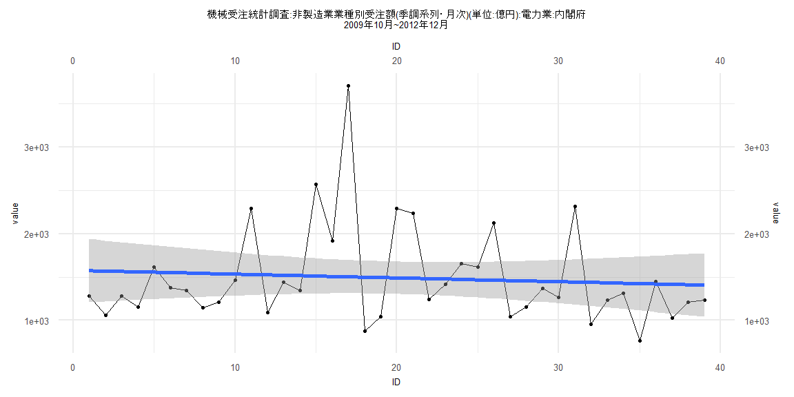
Call:
lm(formula = value ~ ID)

Residuals:
   Min     1Q Median     3Q    Max
-659.5 -359.5 -177.8  105.6 2202.2

Coefficients:
            Estimate Std. Error t value       Pr(>|t|)
(Intercept) 1577.952    187.730   8.405 0.000000000417 ***
ID            -4.364      8.180  -0.534          0.597
---
Signif. codes:  0 '***' 0.001 '**' 0.01 '*' 0.05 '.' 0.1 ' ' 1

Residual standard error: 574.9 on 37 degrees of freedom
Multiple R-squared:  0.007634,  Adjusted R-squared:  -0.01919
F-statistic: 0.2846 on 1 and 37 DF,  p-value: 0.5969


    Two-sample Kolmogorov-Smirnov test

data:  lm_residuals and rnorm(n = length(lm_residuals), mean = 0, sd = sd(lm_residuals))
D = 0.25641, p-value = 0.1547
alternative hypothesis: two-sided


    Durbin-Watson test

data:  value ~ ID
DW = 1.9668, p-value = 0.3909
alternative hypothesis: true autocorrelation is greater than 0


    studentized Breusch-Pagan test

data:  value ~ ID
BP = 0.07429, df = 1, p-value = 0.7852


    Box-Ljung test

data:  lm_residuals
X-squared = 0.0060172, df = 1, p-value = 0.9382
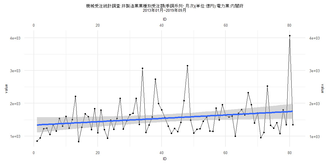
Call:
lm(formula = value ~ ID)

Residuals:
   Min     1Q Median     3Q    Max
-750.8 -338.1 -105.7  166.1 2315.4

Coefficients:
            Estimate Std. Error t value            Pr(>|t|)
(Intercept) 1337.043    117.733  11.357 <0.0000000000000002 ***
ID             5.158      2.494   2.068              0.0419 *
---
Signif. codes:  0 '***' 0.001 '**' 0.01 '*' 0.05 '.' 0.1 ' ' 1

Residual standard error: 524.9 on 79 degrees of freedom
Multiple R-squared:  0.05134,   Adjusted R-squared:  0.03933
F-statistic: 4.276 on 1 and 79 DF,  p-value: 0.04194


    Two-sample Kolmogorov-Smirnov test

data:  lm_residuals and rnorm(n = length(lm_residuals), mean = 0, sd = sd(lm_residuals))
D = 0.22222, p-value = 0.03633
alternative hypothesis: two-sided


    Durbin-Watson test

data:  value ~ ID
DW = 2.0488, p-value = 0.542
alternative hypothesis: true autocorrelation is greater than 0


    studentized Breusch-Pagan test

data:  value ~ ID
BP = 2.9974, df = 1, p-value = 0.0834


    Box-Ljung test

data:  lm_residuals
X-squared = 0.096361, df = 1, p-value = 0.7562
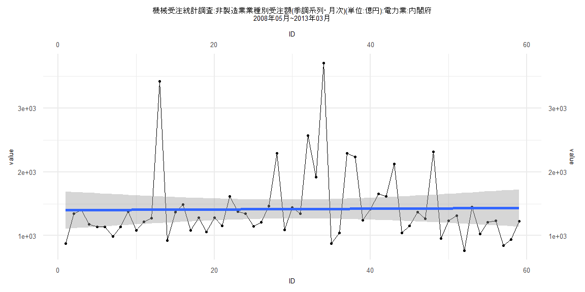
Call:
lm(formula = value ~ ID)

Residuals:
    Min      1Q  Median      3Q     Max
-664.08 -299.07 -161.27   21.82 2286.64

Coefficients:
             Estimate Std. Error t value         Pr(>|t|)
(Intercept) 1399.5648   150.0259   9.329 0.00000000000045 ***
ID             0.5817     4.3490   0.134            0.894
---
Signif. codes:  0 '***' 0.001 '**' 0.01 '*' 0.05 '.' 0.1 ' ' 1

Residual standard error: 568.9 on 57 degrees of freedom
Multiple R-squared:  0.0003138, Adjusted R-squared:  -0.01722
F-statistic: 0.01789 on 1 and 57 DF,  p-value: 0.8941


    Two-sample Kolmogorov-Smirnov test

data:  lm_residuals and rnorm(n = length(lm_residuals), mean = 0, sd = sd(lm_residuals))
D = 0.28814, p-value = 0.01452
alternative hypothesis: two-sided


    Durbin-Watson test

data:  value ~ ID
DW = 1.9548, p-value = 0.3777
alternative hypothesis: true autocorrelation is greater than 0


    studentized Breusch-Pagan test

data:  value ~ ID
BP = 0.000042647, df = 1, p-value = 0.9948


    Box-Ljung test

data:  lm_residuals
X-squared = 0.01227, df = 1, p-value = 0.9118
Call:
lm(formula = value ~ ID)

Residuals:
    Min      1Q  Median      3Q     Max
-733.76 -358.85  -90.68  157.63 2341.95

Coefficients:
            Estimate Std. Error t value            Pr(>|t|)
(Intercept) 1407.481    121.003   11.63 <0.0000000000000002 ***
ID             4.099      2.661    1.54               0.128
---
Signif. codes:  0 '***' 0.001 '**' 0.01 '*' 0.05 '.' 0.1 ' ' 1

Residual standard error: 529.2 on 76 degrees of freedom
Multiple R-squared:  0.03027,   Adjusted R-squared:  0.01751
F-statistic: 2.372 on 1 and 76 DF,  p-value: 0.1277


    Two-sample Kolmogorov-Smirnov test

data:  lm_residuals and rnorm(n = length(lm_residuals), mean = 0, sd = sd(lm_residuals))
D = 0.15385, p-value = 0.316
alternative hypothesis: two-sided


    Durbin-Watson test

data:  value ~ ID
DW = 2.0911, p-value = 0.6129
alternative hypothesis: true autocorrelation is greater than 0


    studentized Breusch-Pagan test

data:  value ~ ID
BP = 2.7954, df = 1, p-value = 0.09453


    Box-Ljung test

data:  lm_residuals
X-squared = 0.19992, df = 1, p-value = 0.6548