Analysis
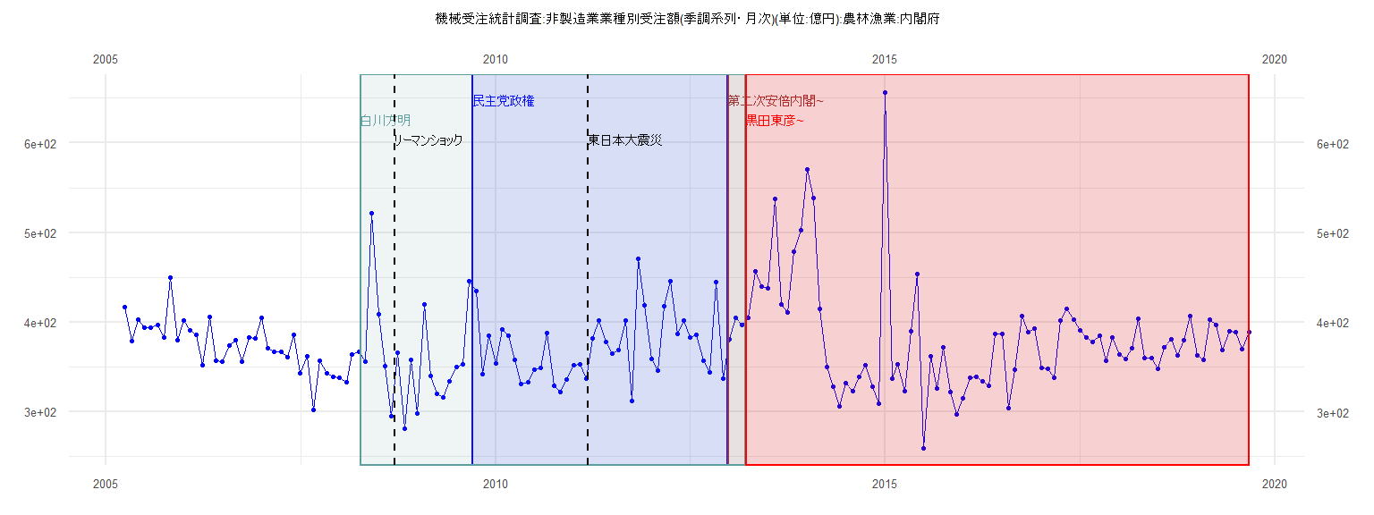
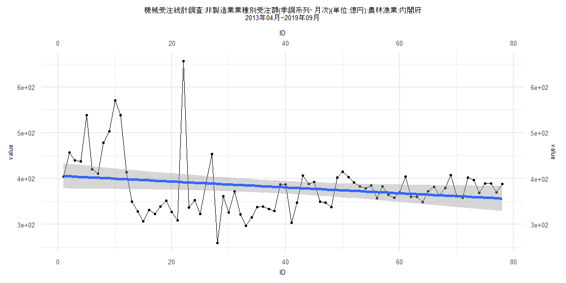
[1] "機械受注統計調査:非製造業業種別受注額(季調系列・月次)(単位:億円):農林漁業:内閣府"
        Jan    Feb    Mar    Apr    May    Jun    Jul    Aug    Sep    Oct    Nov    Dec
2005                      416.57 378.78 402.96 394.22 393.45 396.47 382.73 449.87 379.98
2006 401.33 391.01 386.32 351.92 405.70 356.55 355.62 373.67 380.27 355.77 382.50 382.33
2007 404.89 370.57 366.65 366.56 360.79 385.50 343.33 361.45 301.50 357.06 342.51 338.89
2008 337.95 332.60 363.49 366.39 355.54 522.02 408.43 350.68 294.73 366.31 281.06 357.72
2009 297.83 420.25 339.54 320.06 316.38 333.64 349.42 353.27 445.54 435.04 341.49 384.86
2010 353.84 392.23 385.29 357.83 331.19 332.73 346.62 349.22 387.51 329.00 321.72 336.37
2011 351.83 352.65 336.75 381.62 401.72 377.76 364.42 368.37 401.78 312.17 471.16 419.00
2012 358.87 346.03 417.55 446.12 387.11 401.49 382.74 385.82 357.20 343.72 444.55 337.04
2013 380.70 404.38 396.56 404.64 456.45 439.49 437.26 537.91 420.19 410.96 478.36 502.76
2014 570.90 538.32 414.30 349.96 328.30 306.15 331.75 322.80 339.04 352.22 327.52 308.85
2015 656.26 336.53 352.74 322.79 389.83 453.51 259.52 361.68 325.53 371.69 321.97 297.06
2016 314.92 337.47 339.35 333.81 329.42 387.29 386.98 303.94 347.14 406.74 388.50 392.91
2017 349.40 347.85 337.86 402.30 414.85 403.21 390.92 382.37 378.23 384.99 357.01 382.51
2018 364.12 358.60 370.37 404.25 359.94 359.82 348.36 371.72 381.33 363.21 379.81 407.14
2019 362.62 357.67 402.33 396.97 369.30 389.46 388.81 369.53 388.61
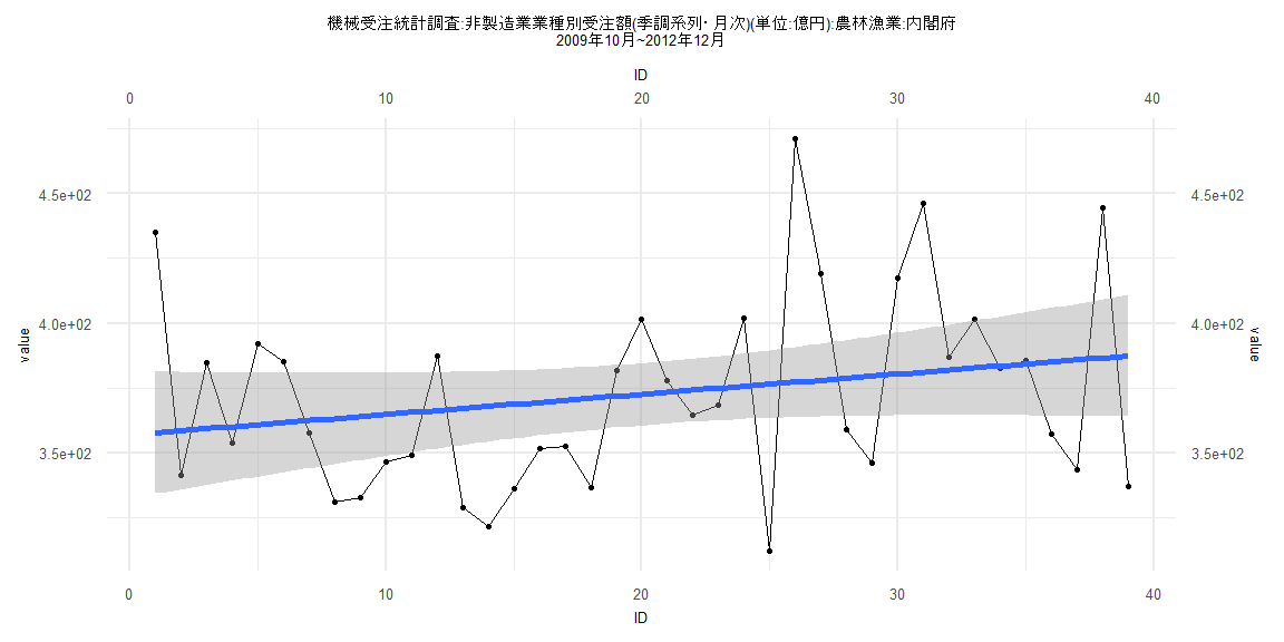
Call:
lm(formula = value ~ ID)

Residuals:
    Min      1Q  Median      3Q     Max
-64.360 -29.613  -6.293  24.551  93.849

Coefficients:
            Estimate Std. Error t value            Pr(>|t|)
(Intercept) 357.0102    12.0453  29.639 <0.0000000000000002 ***
ID            0.7808     0.5249   1.488               0.145
---
Signif. codes:  0 '***' 0.001 '**' 0.01 '*' 0.05 '.' 0.1 ' ' 1

Residual standard error: 36.89 on 37 degrees of freedom
Multiple R-squared:  0.05643,   Adjusted R-squared:  0.03093
F-statistic: 2.213 on 1 and 37 DF,  p-value: 0.1453


    Two-sample Kolmogorov-Smirnov test

data:  lm_residuals and rnorm(n = length(lm_residuals), mean = 0, sd = sd(lm_residuals))
D = 0.17949, p-value = 0.5622
alternative hypothesis: two-sided


    Durbin-Watson test

data:  value ~ ID
DW = 1.9348, p-value = 0.3528
alternative hypothesis: true autocorrelation is greater than 0


    studentized Breusch-Pagan test

data:  value ~ ID
BP = 0.62407, df = 1, p-value = 0.4295


    Box-Ljung test

data:  lm_residuals
X-squared = 0.11341, df = 1, p-value = 0.7363
Call:
lm(formula = value ~ ID)

Residuals:
     Min       1Q   Median       3Q      Max
-128.026  -40.753    0.814   27.416  265.096

Coefficients:
            Estimate Std. Error t value            Pr(>|t|)
(Intercept) 406.2383    13.5164  30.055 <0.0000000000000002 ***
ID           -0.6030     0.2864  -2.106              0.0384 *
---
Signif. codes:  0 '***' 0.001 '**' 0.01 '*' 0.05 '.' 0.1 ' ' 1

Residual standard error: 60.26 on 79 degrees of freedom
Multiple R-squared:  0.05314,   Adjusted R-squared:  0.04115
F-statistic: 4.433 on 1 and 79 DF,  p-value: 0.03842


    Two-sample Kolmogorov-Smirnov test

data:  lm_residuals and rnorm(n = length(lm_residuals), mean = 0, sd = sd(lm_residuals))
D = 0.12346, p-value = 0.5705
alternative hypothesis: two-sided


    Durbin-Watson test

data:  value ~ ID
DW = 1.3427, p-value = 0.0007593
alternative hypothesis: true autocorrelation is greater than 0


    studentized Breusch-Pagan test

data:  value ~ ID
BP = 6.2375, df = 1, p-value = 0.01251


    Box-Ljung test

data:  lm_residuals
X-squared = 8.9242, df = 1, p-value = 0.002814
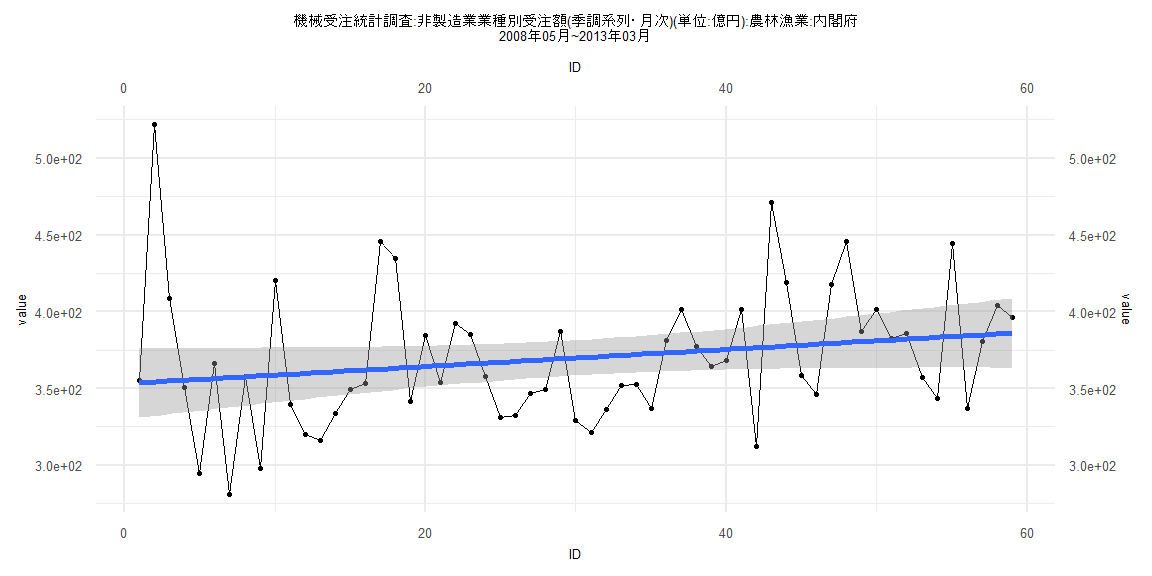
Call:
lm(formula = value ~ ID)

Residuals:
    Min      1Q  Median      3Q     Max
-76.040 -30.105  -7.153  19.821 167.711

Coefficients:
            Estimate Std. Error t value            Pr(>|t|)
(Intercept) 353.1925    11.6365  30.352 <0.0000000000000002 ***
ID            0.5583     0.3373   1.655               0.103
---
Signif. codes:  0 '***' 0.001 '**' 0.01 '*' 0.05 '.' 0.1 ' ' 1

Residual standard error: 44.12 on 57 degrees of freedom
Multiple R-squared:  0.04585,   Adjusted R-squared:  0.02911
F-statistic: 2.739 on 1 and 57 DF,  p-value: 0.1034


    Two-sample Kolmogorov-Smirnov test

data:  lm_residuals and rnorm(n = length(lm_residuals), mean = 0, sd = sd(lm_residuals))
D = 0.084746, p-value = 0.9854
alternative hypothesis: two-sided


    Durbin-Watson test

data:  value ~ ID
DW = 1.8001, p-value = 0.1812
alternative hypothesis: true autocorrelation is greater than 0


    studentized Breusch-Pagan test

data:  value ~ ID
BP = 3.4049, df = 1, p-value = 0.065


    Box-Ljung test

data:  lm_residuals
X-squared = 0.61358, df = 1, p-value = 0.4334
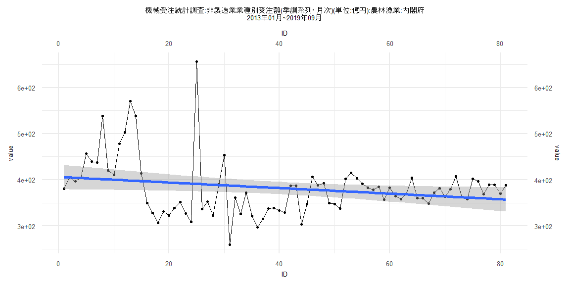
Call:
lm(formula = value ~ ID)

Residuals:
     Min       1Q   Median       3Q      Max
-128.854  -43.415    1.715   27.778  264.060

Coefficients:
            Estimate Std. Error t value            Pr(>|t|)
(Intercept) 406.2290    14.0298  28.955 <0.0000000000000002 ***
ID           -0.6377     0.3086  -2.067              0.0422 *
---
Signif. codes:  0 '***' 0.001 '**' 0.01 '*' 0.05 '.' 0.1 ' ' 1

Residual standard error: 61.36 on 76 degrees of freedom
Multiple R-squared:  0.0532,    Adjusted R-squared:  0.04074
F-statistic:  4.27 on 1 and 76 DF,  p-value: 0.04219


    Two-sample Kolmogorov-Smirnov test

data:  lm_residuals and rnorm(n = length(lm_residuals), mean = 0, sd = sd(lm_residuals))
D = 0.19231, p-value = 0.1118
alternative hypothesis: two-sided


    Durbin-Watson test

data:  value ~ ID
DW = 1.3437, p-value = 0.0009289
alternative hypothesis: true autocorrelation is greater than 0


    studentized Breusch-Pagan test

data:  value ~ ID
BP = 7.9404, df = 1, p-value = 0.004834


    Box-Ljung test

data:  lm_residuals
X-squared = 8.631, df = 1, p-value = 0.003305