Analysis
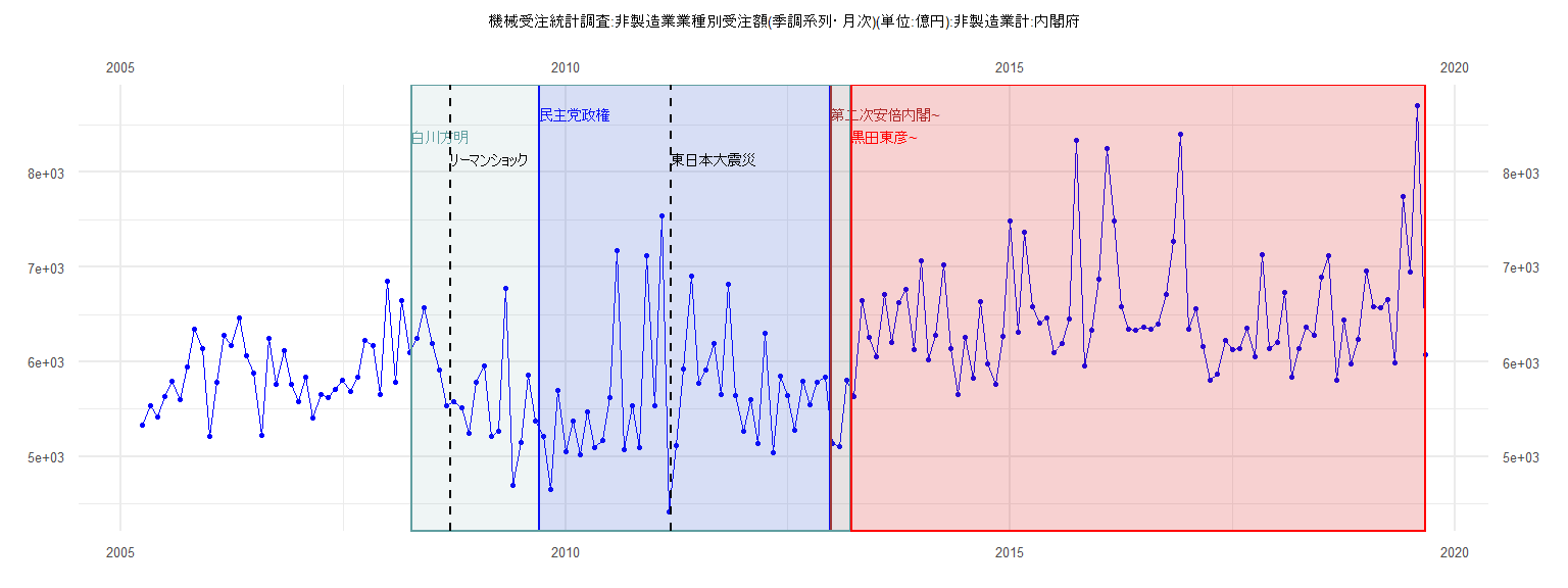
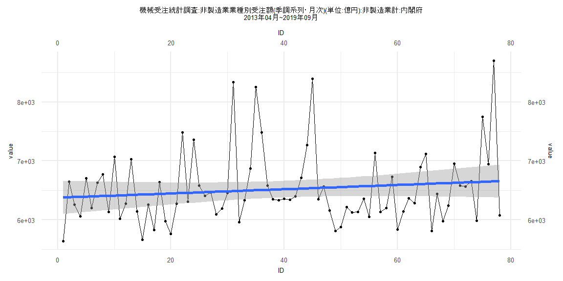
[1] "機械受注統計調査:非製造業業種別受注額(季調系列・月次)(単位:億円):非製造業計:内閣府"
         Jan     Feb     Mar     Apr     May     Jun     Jul     Aug     Sep     Oct     Nov     Dec
2005                         5327.76 5535.57 5414.58 5634.51 5790.08 5600.52 5943.71 6346.58 6134.67
2006 5216.78 5782.56 6278.53 6172.31 6467.47 6063.45 5879.07 5229.18 6242.86 5766.81 6118.49 5757.73
2007 5584.58 5842.40 5403.22 5659.98 5619.00 5713.97 5802.86 5689.73 5833.71 6225.29 6169.76 5657.40
2008 6846.15 5779.66 6644.24 6095.10 6244.68 6570.00 6191.89 5914.74 5540.48 5581.77 5517.68 5244.67
2009 5788.58 5960.48 5210.14 5265.36 6776.93 4695.46 5147.41 5859.78 5370.51 5214.29 4650.72 5702.66
2010 5046.89 5379.74 5020.62 5472.37 5090.32 5168.68 5618.36 7177.86 5076.59 5539.67 5100.09 7124.23
2011 5535.40 7538.01 4421.84 5113.79 5923.28 6908.28 5768.63 5909.58 6194.32 5651.91 6818.91 5639.85
2012 5264.95 5596.04 5135.81 6305.42 5043.21 5846.05 5644.99 5283.17 5800.40 5542.79 5782.20 5835.71
2013 5141.77 5101.99 5807.53 5637.93 6650.56 6262.42 6058.84 6706.06 6198.88 6627.68 6769.34 6133.09
2014 7066.60 6018.50 6277.25 7024.81 6144.69 5660.10 6261.60 5828.12 6638.26 5979.50 5763.25 6272.74
2015 7484.71 6306.64 7362.37 6578.21 6405.50 6463.35 6095.91 6190.50 6456.35 8338.40 5956.48 6329.37
2016 6869.53 8251.55 7484.19 6583.97 6345.97 6334.27 6361.93 6343.46 6396.76 6711.46 7267.72 8396.38
2017 6348.36 6561.56 6155.95 5809.83 5875.18 6220.79 6127.33 6136.16 6355.93 6050.87 7133.16 6134.76
2018 6202.90 6730.19 5837.81 6139.72 6363.94 6283.06 6897.44 7119.88 5808.65 6441.15 5979.02 6240.41
2019 6952.75 6584.73 6568.63 6653.09 5985.60 7749.11 6945.82 8701.39 6079.37
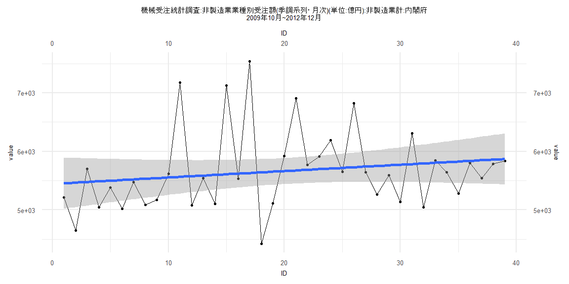
Call:
lm(formula = value ~ ID)

Residuals:
     Min       1Q   Median       3Q      Max
-1220.11  -464.31   -84.71   148.02  1906.98

Coefficients:
            Estimate Std. Error t value            Pr(>|t|)
(Intercept) 5445.416    223.941  24.316 <0.0000000000000002 ***
ID            10.918      9.758   1.119                0.27
---
Signif. codes:  0 '***' 0.001 '**' 0.01 '*' 0.05 '.' 0.1 ' ' 1

Residual standard error: 685.9 on 37 degrees of freedom
Multiple R-squared:  0.03273,   Adjusted R-squared:  0.006587
F-statistic: 1.252 on 1 and 37 DF,  p-value: 0.2704


    Two-sample Kolmogorov-Smirnov test

data:  lm_residuals and rnorm(n = length(lm_residuals), mean = 0, sd = sd(lm_residuals))
D = 0.38462, p-value = 0.00581
alternative hypothesis: two-sided


    Durbin-Watson test

data:  value ~ ID
DW = 2.3801, p-value = 0.8499
alternative hypothesis: true autocorrelation is greater than 0


    studentized Breusch-Pagan test

data:  value ~ ID
BP = 0.63329, df = 1, p-value = 0.4262


    Box-Ljung test

data:  lm_residuals
X-squared = 1.5474, df = 1, p-value = 0.2135
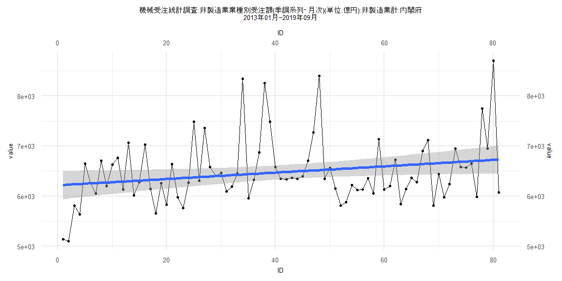
Call:
lm(formula = value ~ ID)

Residuals:
    Min      1Q  Median      3Q     Max
-1127.1  -427.9  -121.8   257.6  1979.3

Coefficients:
            Estimate Std. Error t value            Pr(>|t|)
(Intercept) 6216.460    144.368  43.060 <0.0000000000000002 ***
ID             6.320      3.059   2.066              0.0421 *
---
Signif. codes:  0 '***' 0.001 '**' 0.01 '*' 0.05 '.' 0.1 ' ' 1

Residual standard error: 643.6 on 79 degrees of freedom
Multiple R-squared:  0.05127,   Adjusted R-squared:  0.03926
F-statistic: 4.269 on 1 and 79 DF,  p-value: 0.0421


    Two-sample Kolmogorov-Smirnov test

data:  lm_residuals and rnorm(n = length(lm_residuals), mean = 0, sd = sd(lm_residuals))
D = 0.12346, p-value = 0.5705
alternative hypothesis: two-sided


    Durbin-Watson test

data:  value ~ ID
DW = 1.648, p-value = 0.04288
alternative hypothesis: true autocorrelation is greater than 0


    studentized Breusch-Pagan test

data:  value ~ ID
BP = 0.34611, df = 1, p-value = 0.5563


    Box-Ljung test

data:  lm_residuals
X-squared = 1.9346, df = 1, p-value = 0.1643
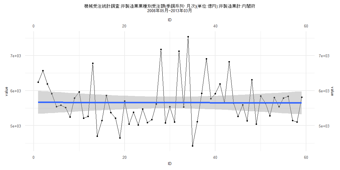
Call:
lm(formula = value ~ ID)

Residuals:
     Min       1Q   Median       3Q      Max
-1234.81  -471.55   -82.46   224.08  1881.10

Coefficients:
             Estimate Std. Error t value            Pr(>|t|)
(Intercept) 5665.7949   168.8091  33.563 <0.0000000000000002 ***
ID            -0.2613     4.8935  -0.053               0.958
---
Signif. codes:  0 '***' 0.001 '**' 0.01 '*' 0.05 '.' 0.1 ' ' 1

Residual standard error: 640.1 on 57 degrees of freedom
Multiple R-squared:  5e-05, Adjusted R-squared:  -0.01749
F-statistic: 0.00285 on 1 and 57 DF,  p-value: 0.9576


    Two-sample Kolmogorov-Smirnov test

data:  lm_residuals and rnorm(n = length(lm_residuals), mean = 0, sd = sd(lm_residuals))
D = 0.18644, p-value = 0.2582
alternative hypothesis: two-sided


    Durbin-Watson test

data:  value ~ ID
DW = 2.2028, p-value = 0.7416
alternative hypothesis: true autocorrelation is greater than 0


    studentized Breusch-Pagan test

data:  value ~ ID
BP = 0.048223, df = 1, p-value = 0.8262


    Box-Ljung test

data:  lm_residuals
X-squared = 0.73849, df = 1, p-value = 0.3901
Call:
lm(formula = value ~ ID)

Residuals:
   Min     1Q Median     3Q    Max
-805.7 -391.3 -166.8  256.6 2047.4

Coefficients:
            Estimate Std. Error t value            Pr(>|t|)
(Intercept) 6376.518    142.998  44.592 <0.0000000000000002 ***
ID             3.603      3.145   1.146               0.256
---
Signif. codes:  0 '***' 0.001 '**' 0.01 '*' 0.05 '.' 0.1 ' ' 1

Residual standard error: 625.4 on 76 degrees of freedom
Multiple R-squared:  0.01698,   Adjusted R-squared:  0.004041
F-statistic: 1.312 on 1 and 76 DF,  p-value: 0.2555


    Two-sample Kolmogorov-Smirnov test

data:  lm_residuals and rnorm(n = length(lm_residuals), mean = 0, sd = sd(lm_residuals))
D = 0.17949, p-value = 0.1624
alternative hypothesis: two-sided


    Durbin-Watson test

data:  value ~ ID
DW = 1.7969, p-value = 0.1538
alternative hypothesis: true autocorrelation is greater than 0


    studentized Breusch-Pagan test

data:  value ~ ID
BP = 1.0731, df = 1, p-value = 0.3002


    Box-Ljung test

data:  lm_residuals
X-squared = 0.60859, df = 1, p-value = 0.4353