Analysis
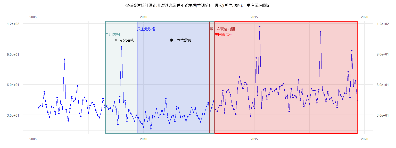
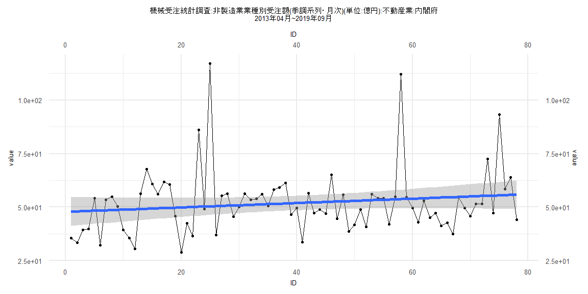
[1] "機械受注統計調査:非製造業業種別受注額(季調系列・月次)(単位:億円):不動産業:内閣府"
Jan Feb Mar Apr May Jun Jul Aug Sep Oct Nov Dec
2005 37.12 39.19 38.42 52.86 40.10 32.30 27.96 38.64 37.30
2006 30.33 47.40 31.52 43.77 35.62 85.06 35.35 24.28 36.15 48.22 43.35 45.77
2007 59.21 31.37 28.76 44.76 47.42 43.88 31.96 39.19 42.23 40.51 34.63 30.07
2008 27.31 34.62 46.57 37.20 38.93 35.93 37.01 33.83 42.86 35.80 20.54 48.15
2009 97.53 42.83 44.58 23.95 35.59 31.88 28.62 23.92 29.88 27.77 23.21 21.85
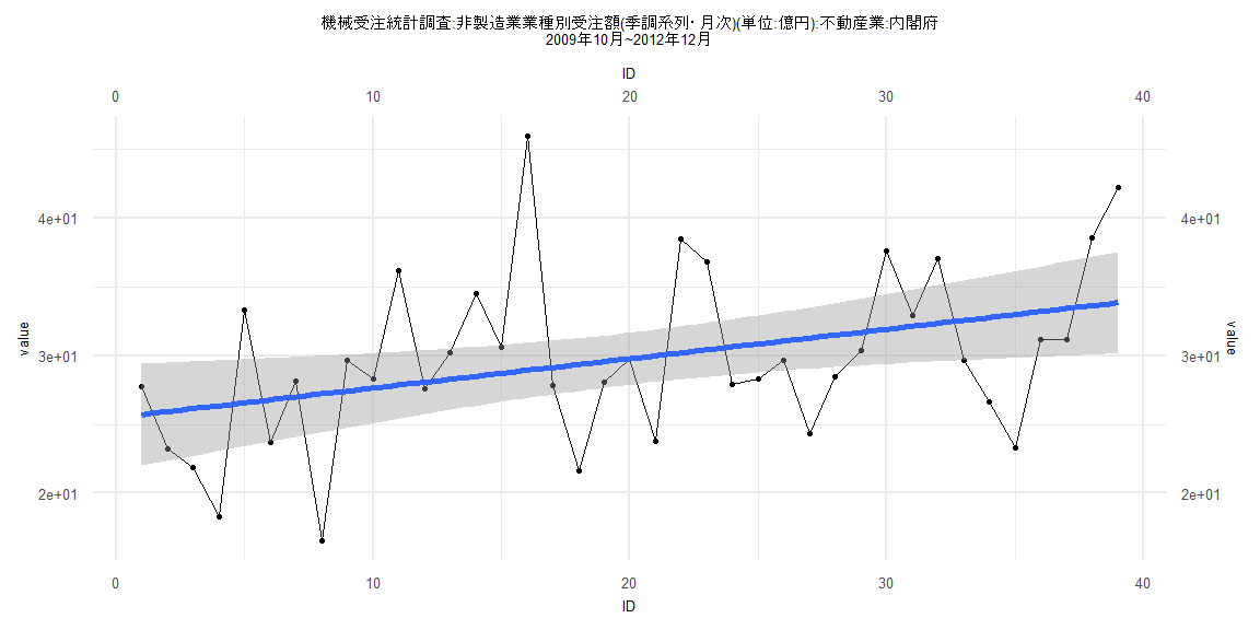
2010 18.27 33.29 23.67 28.13 16.54 29.63 28.31 36.17 27.59 30.22 34.52 30.57
2011 45.95 27.81 21.66 28.10 29.71 23.78 38.51 36.79 27.94 28.34 29.64 24.35
2012 28.48 30.36 37.64 32.89 37.02 29.67 26.60 23.28 31.17 31.16 38.54 42.18
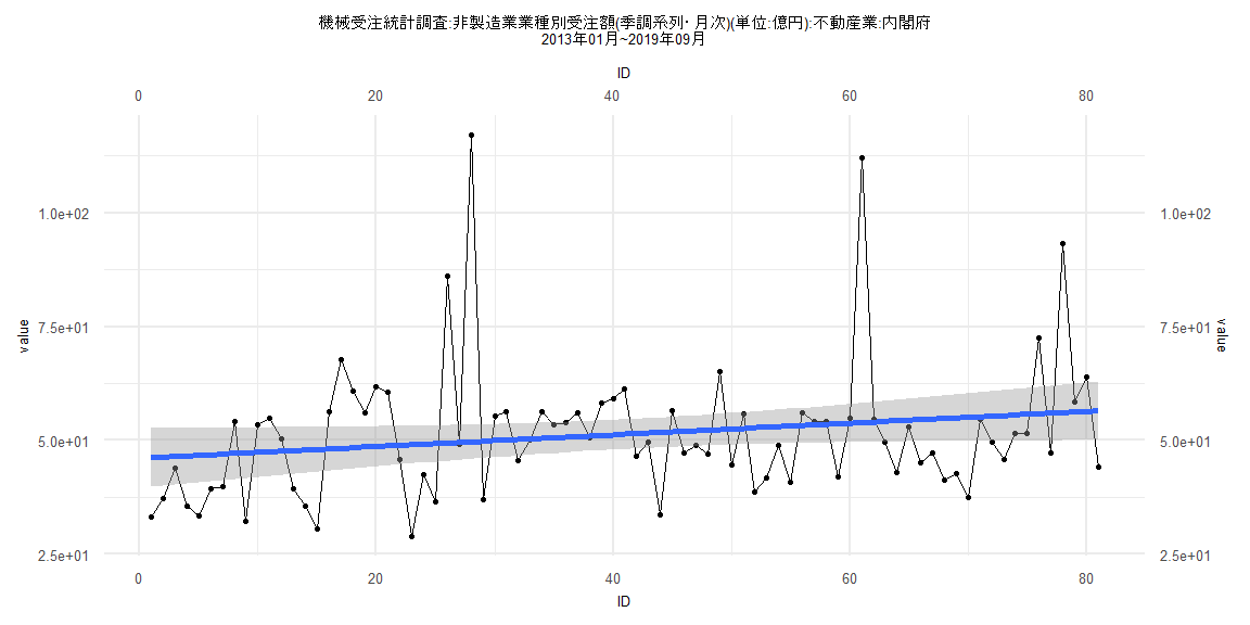
2013 33.24 37.15 43.80 35.45 33.35 39.43 39.74 54.17 32.15 53.39 54.90 50.37
2014 39.30 35.46 30.59 56.29 67.69 60.74 56.14 61.86 60.50 45.71 28.89 42.42
2015 36.41 86.19 49.12 117.06 37.00 55.33 56.38 45.65 49.98 56.34 53.47 53.81
2016 56.00 50.65 58.22 59.13 61.27 46.62 49.65 33.62 56.42 47.14 48.96 47.04
2017 65.13 44.69 55.73 38.63 41.82 48.83 40.85 56.07 54.04 54.08 42.09 54.77
2018 111.99 54.63 49.72 42.96 53.03 45.18 47.31 41.17 42.73 37.51 54.60 49.70
2019 45.78 51.51 51.51 72.48 47.29 93.31 58.37 63.98 44.25
Call:
lm(formula = value ~ ID)

Residuals:
    Min      1Q  Median      3Q     Max
-10.668  -2.950  -1.325   3.441  17.029

Coefficients:
            Estimate Std. Error t value             Pr(>|t|)
(Intercept) 25.49459    1.90380  13.391 0.000000000000000923 ***
ID           0.21413    0.08296   2.581               0.0139 *
---
Signif. codes:  0 '***' 0.001 '**' 0.01 '*' 0.05 '.' 0.1 ' ' 1

Residual standard error: 5.831 on 37 degrees of freedom
Multiple R-squared:  0.1526,    Adjusted R-squared:  0.1297
F-statistic: 6.663 on 1 and 37 DF,  p-value: 0.01394


    Two-sample Kolmogorov-Smirnov test

data:  lm_residuals and rnorm(n = length(lm_residuals), mean = 0, sd = sd(lm_residuals))
D = 0.12821, p-value = 0.9114
alternative hypothesis: two-sided


    Durbin-Watson test

data:  value ~ ID
DW = 1.7341, p-value = 0.1551
alternative hypothesis: true autocorrelation is greater than 0


    studentized Breusch-Pagan test

data:  value ~ ID
BP = 0.032408, df = 1, p-value = 0.8571


    Box-Ljung test

data:  lm_residuals
X-squared = 0.45201, df = 1, p-value = 0.5014
Call:
lm(formula = value ~ ID)

Residuals:
    Min      1Q  Median      3Q     Max
-20.156  -9.388  -2.677   5.882  67.372

Coefficients:
            Estimate Std. Error t value            Pr(>|t|)
(Intercept) 46.09207    3.32205  13.875 <0.0000000000000002 ***
ID           0.12842    0.07039   1.824              0.0719 .
---
Signif. codes:  0 '***' 0.001 '**' 0.01 '*' 0.05 '.' 0.1 ' ' 1

Residual standard error: 14.81 on 79 degrees of freedom
Multiple R-squared:  0.04043,   Adjusted R-squared:  0.02829
F-statistic: 3.329 on 1 and 79 DF,  p-value: 0.07186


    Two-sample Kolmogorov-Smirnov test

data:  lm_residuals and rnorm(n = length(lm_residuals), mean = 0, sd = sd(lm_residuals))
D = 0.18519, p-value = 0.1245
alternative hypothesis: two-sided


    Durbin-Watson test

data:  value ~ ID
DW = 1.9382, p-value = 0.3467
alternative hypothesis: true autocorrelation is greater than 0


    studentized Breusch-Pagan test

data:  value ~ ID
BP = 0.012696, df = 1, p-value = 0.9103


    Box-Ljung test

data:  lm_residuals
X-squared = 0.039564, df = 1, p-value = 0.8423
Call:
lm(formula = value ~ ID)

Residuals:
    Min      1Q  Median      3Q     Max
-16.574  -5.120  -1.863   3.496  62.983

Coefficients:
            Estimate Std. Error t value            Pr(>|t|)
(Intercept) 35.35278    2.92797  12.074 <0.0000000000000002 ***
ID          -0.08954    0.08488  -1.055               0.296
---
Signif. codes:  0 '***' 0.001 '**' 0.01 '*' 0.05 '.' 0.1 ' ' 1

Residual standard error: 11.1 on 57 degrees of freedom
Multiple R-squared:  0.01915,   Adjusted R-squared:  0.001942
F-statistic: 1.113 on 1 and 57 DF,  p-value: 0.2959


    Two-sample Kolmogorov-Smirnov test

data:  lm_residuals and rnorm(n = length(lm_residuals), mean = 0, sd = sd(lm_residuals))
D = 0.11864, p-value = 0.8052
alternative hypothesis: two-sided


    Durbin-Watson test

data:  value ~ ID
DW = 1.3599, p-value = 0.003703
alternative hypothesis: true autocorrelation is greater than 0


    studentized Breusch-Pagan test

data:  value ~ ID
BP = 1.8168, df = 1, p-value = 0.1777


    Box-Ljung test

data:  lm_residuals
X-squared = 5.799, df = 1, p-value = 0.01604
Call:
lm(formula = value ~ ID)

Residuals:
    Min      1Q  Median      3Q     Max
-20.976  -9.191  -1.713   5.223  66.681

Coefficients:
            Estimate Std. Error t value            Pr(>|t|)
(Intercept) 47.81198    3.42329  13.967 <0.0000000000000002 ***
ID           0.10270    0.07529   1.364               0.177
---
Signif. codes:  0 '***' 0.001 '**' 0.01 '*' 0.05 '.' 0.1 ' ' 1

Residual standard error: 14.97 on 76 degrees of freedom
Multiple R-squared:  0.02389,   Adjusted R-squared:  0.01105
F-statistic:  1.86 on 1 and 76 DF,  p-value: 0.1766


    Two-sample Kolmogorov-Smirnov test

data:  lm_residuals and rnorm(n = length(lm_residuals), mean = 0, sd = sd(lm_residuals))
D = 0.16667, p-value = 0.2297
alternative hypothesis: two-sided


    Durbin-Watson test

data:  value ~ ID
DW = 1.9642, p-value = 0.3911
alternative hypothesis: true autocorrelation is greater than 0


    studentized Breusch-Pagan test

data:  value ~ ID
BP = 0.00020783, df = 1, p-value = 0.9885


    Box-Ljung test

data:  lm_residuals
X-squared = 0.0072004, df = 1, p-value = 0.9324