Analysis
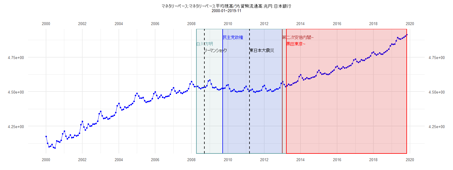
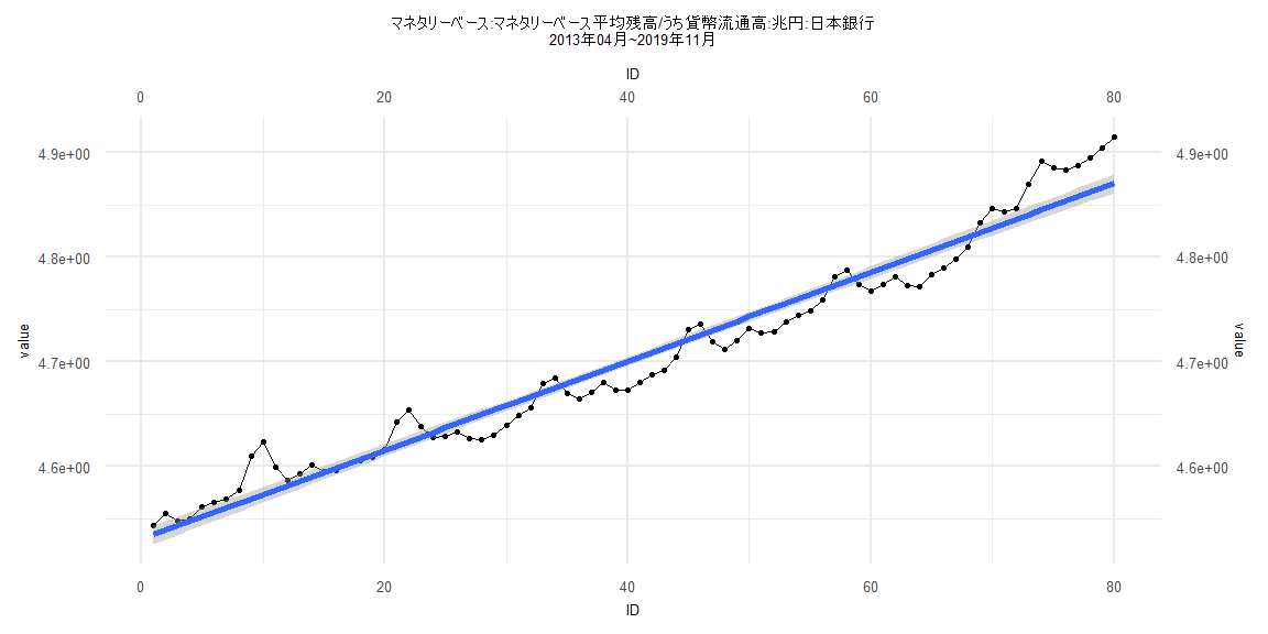
[1] "マネタリーベース:マネタリーベース平均残高/うち貨幣流通高:兆円:日本銀行"
        Jan    Feb    Mar    Apr    May    Jun    Jul    Aug    Sep    Oct    Nov    Dec
2000 4.1749 4.1270 4.1009 4.1052 4.1183 4.0955 4.0914 4.1439 4.1391 4.1352 4.1465 4.1939
2001 4.2134 4.1773 4.1579 4.1687 4.1857 4.1665 4.1691 4.1834 4.1797 4.1832 4.1996 4.2604
2002 4.2843 4.2446 4.2216 4.2374 4.2649 4.2506 4.2522 4.2653 4.2663 4.2692 4.2876 4.3398
2003 4.3584 4.3246 4.3051 4.3077 4.3143 4.3016 4.3059 4.3207 4.3240 4.3303 4.3485 4.3990
2004 4.4148 4.3851 4.3681 4.3715 4.3889 4.3829 4.3871 4.4011 4.4061 4.4163 4.4309 4.4734
2005 4.4871 4.4683 4.4540 4.4529 4.4573 4.4349 4.4233 4.4288 4.4299 4.4345 4.4491 4.4859
2006 4.4987 4.4724 4.4521 4.4619 4.4760 4.4600 4.4555 4.4647 4.4658 4.4691 4.4822 4.5143
2007 4.5280 4.5061 4.4902 4.4972 4.5064 4.4914 4.4884 4.4972 4.5002 4.5071 4.5215 4.5575
2008 4.5739 4.5513 4.5363 4.5371 4.5404 4.5281 4.5232 4.5280 4.5301 4.5329 4.5434 4.5770
2009 4.5846 4.5568 4.5308 4.5280 4.5326 4.5181 4.5142 4.5186 4.5240 4.5248 4.5270 4.5462
2010 4.5509 4.5233 4.5041 4.5067 4.5153 4.5032 4.4979 4.5033 4.5037 4.5040 4.5096 4.5294
2011 4.5400 4.5171 4.5022 4.5124 4.5187 4.5013 4.4958 4.5028 4.5034 4.5051 4.5106 4.5364
2012 4.5466 4.5215 4.5052 4.5087 4.5149 4.5031 4.5044 4.5143 4.5196 4.5212 4.5285 4.5605
2013 4.5742 4.5522 4.5368 4.5433 4.5549 4.5480 4.5498 4.5611 4.5661 4.5693 4.5774 4.6101
2014 4.6233 4.5994 4.5870 4.5936 4.6013 4.5950 4.5962 4.6025 4.6053 4.6085 4.6161 4.6430
2015 4.6545 4.6378 4.6280 4.6292 4.6335 4.6270 4.6254 4.6302 4.6397 4.6488 4.6563 4.6790
2016 4.6849 4.6694 4.6642 4.6706 4.6799 4.6732 4.6735 4.6808 4.6874 4.6917 4.7042 4.7307
2017 4.7363 4.7193 4.7121 4.7204 4.7319 4.7274 4.7282 4.7386 4.7443 4.7485 4.7595 4.7817
2018 4.7878 4.7741 4.7672 4.7735 4.7812 4.7729 4.7720 4.7830 4.7899 4.7978 4.8095 4.8326
2019 4.8463 4.8433 4.8466 4.8696 4.8918 4.8850 4.8831 4.8876 4.8947 4.9045 4.9147
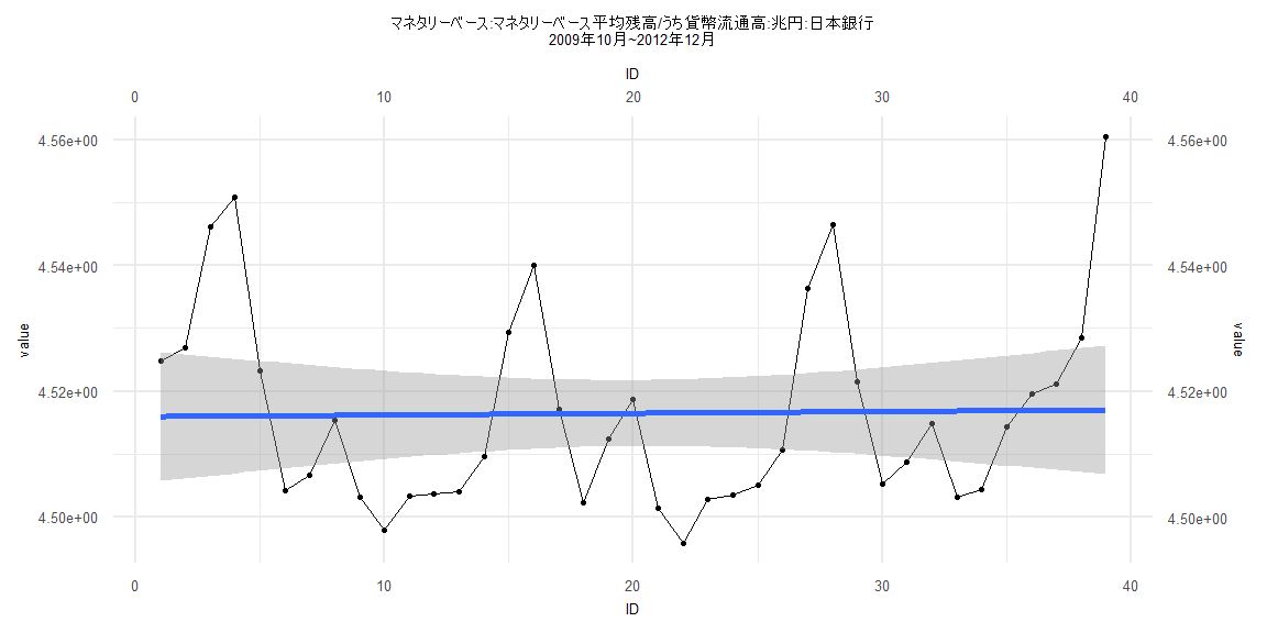
Call:
lm(formula = value ~ ID)

Residuals:
      Min        1Q    Median        3Q       Max
-0.020760 -0.012538 -0.004078  0.008012  0.043473

Coefficients:
              Estimate Std. Error t value            Pr(>|t|)
(Intercept) 4.51595574 0.00528472 854.531 <0.0000000000000002 ***
ID          0.00002747 0.00023028   0.119               0.906
---
Signif. codes:  0 '***' 0.001 '**' 0.01 '*' 0.05 '.' 0.1 ' ' 1

Residual standard error: 0.01619 on 37 degrees of freedom
Multiple R-squared:  0.0003844, Adjusted R-squared:  -0.02663
F-statistic: 0.01423 on 1 and 37 DF,  p-value: 0.9057


    Two-sample Kolmogorov-Smirnov test

data:  lm_residuals and rnorm(n = length(lm_residuals), mean = 0, sd = sd(lm_residuals))
D = 0.23077, p-value = 0.2523
alternative hypothesis: two-sided


    Durbin-Watson test

data:  value ~ ID
DW = 0.6926, p-value = 0.0000004785
alternative hypothesis: true autocorrelation is greater than 0


    studentized Breusch-Pagan test

data:  value ~ ID
BP = 0.017988, df = 1, p-value = 0.8933


    Box-Ljung test

data:  lm_residuals
X-squared = 12.831, df = 1, p-value = 0.000341
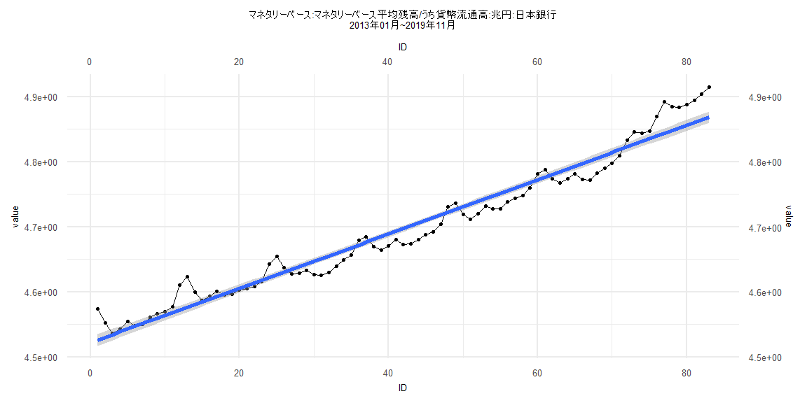
Call:
lm(formula = value ~ ID)

Residuals:
      Min        1Q    Median        3Q       Max
-0.029638 -0.016735 -0.004252  0.009954  0.048404

Coefficients:
              Estimate Std. Error t value            Pr(>|t|)
(Intercept) 4.52186001 0.00459939   983.1 <0.0000000000000002 ***
ID          0.00417579 0.00009512    43.9 <0.0000000000000002 ***
---
Signif. codes:  0 '***' 0.001 '**' 0.01 '*' 0.05 '.' 0.1 ' ' 1

Residual standard error: 0.02076 on 81 degrees of freedom
Multiple R-squared:  0.9597,    Adjusted R-squared:  0.9592
F-statistic:  1927 on 1 and 81 DF,  p-value: < 0.00000000000000022


    Two-sample Kolmogorov-Smirnov test

data:  lm_residuals and rnorm(n = length(lm_residuals), mean = 0, sd = sd(lm_residuals))
D = 0.12048, p-value = 0.5863
alternative hypothesis: two-sided


    Durbin-Watson test

data:  value ~ ID
DW = 0.27958, p-value < 0.00000000000000022
alternative hypothesis: true autocorrelation is greater than 0


    studentized Breusch-Pagan test

data:  value ~ ID
BP = 6.0358, df = 1, p-value = 0.01402


    Box-Ljung test

data:  lm_residuals
X-squared = 54.563, df = 1, p-value = 0.0000000000001505
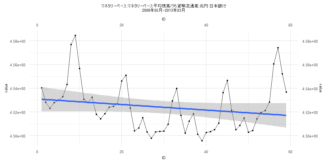
Call:
lm(formula = value ~ ID)

Residuals:
      Min        1Q    Median        3Q       Max
-0.026831 -0.014782 -0.003071  0.007712  0.056490

Coefficients:
              Estimate Std. Error t value            Pr(>|t|)
(Intercept)  4.5310498  0.0053065 853.873 <0.0000000000000002 ***
ID          -0.0002340  0.0001538  -1.521               0.134
---
Signif. codes:  0 '***' 0.001 '**' 0.01 '*' 0.05 '.' 0.1 ' ' 1

Residual standard error: 0.02012 on 57 degrees of freedom
Multiple R-squared:  0.03902,   Adjusted R-squared:  0.02216
F-statistic: 2.315 on 1 and 57 DF,  p-value: 0.1337


    Two-sample Kolmogorov-Smirnov test

data:  lm_residuals and rnorm(n = length(lm_residuals), mean = 0, sd = sd(lm_residuals))
D = 0.13559, p-value = 0.6544
alternative hypothesis: two-sided


    Durbin-Watson test

data:  value ~ ID
DW = 0.47169, p-value = 0.00000000000007107
alternative hypothesis: true autocorrelation is greater than 0


    studentized Breusch-Pagan test

data:  value ~ ID
BP = 0.65402, df = 1, p-value = 0.4187


    Box-Ljung test

data:  lm_residuals
X-squared = 35.266, df = 1, p-value = 0.000000002876
Call:
lm(formula = value ~ ID)

Residuals:
      Min        1Q    Median        3Q       Max
-0.030415 -0.017190 -0.002558  0.010239  0.050247

Coefficients:
              Estimate Std. Error t value            Pr(>|t|)
(Intercept) 4.53057791 0.00455921  993.72 <0.0000000000000002 ***
ID          0.00424746 0.00009779   43.43 <0.0000000000000002 ***
---
Signif. codes:  0 '***' 0.001 '**' 0.01 '*' 0.05 '.' 0.1 ' ' 1

Residual standard error: 0.0202 on 78 degrees of freedom
Multiple R-squared:  0.9603,    Adjusted R-squared:  0.9598
F-statistic:  1886 on 1 and 78 DF,  p-value: < 0.00000000000000022


    Two-sample Kolmogorov-Smirnov test

data:  lm_residuals and rnorm(n = length(lm_residuals), mean = 0, sd = sd(lm_residuals))
D = 0.1375, p-value = 0.4383
alternative hypothesis: two-sided


    Durbin-Watson test

data:  value ~ ID
DW = 0.27285, p-value < 0.00000000000000022
alternative hypothesis: true autocorrelation is greater than 0


    studentized Breusch-Pagan test

data:  value ~ ID
BP = 7.6972, df = 1, p-value = 0.005531


    Box-Ljung test

data:  lm_residuals
X-squared = 57.422, df = 1, p-value = 0.00000000000003519