Analysis
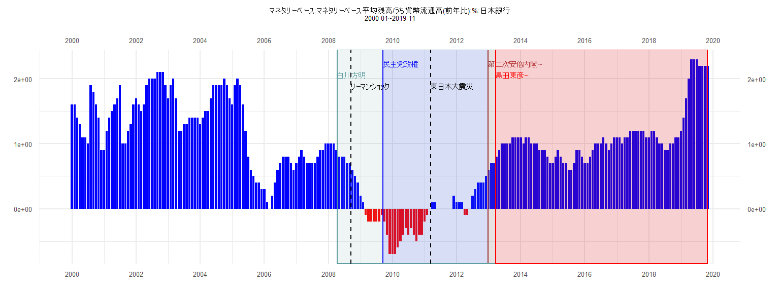
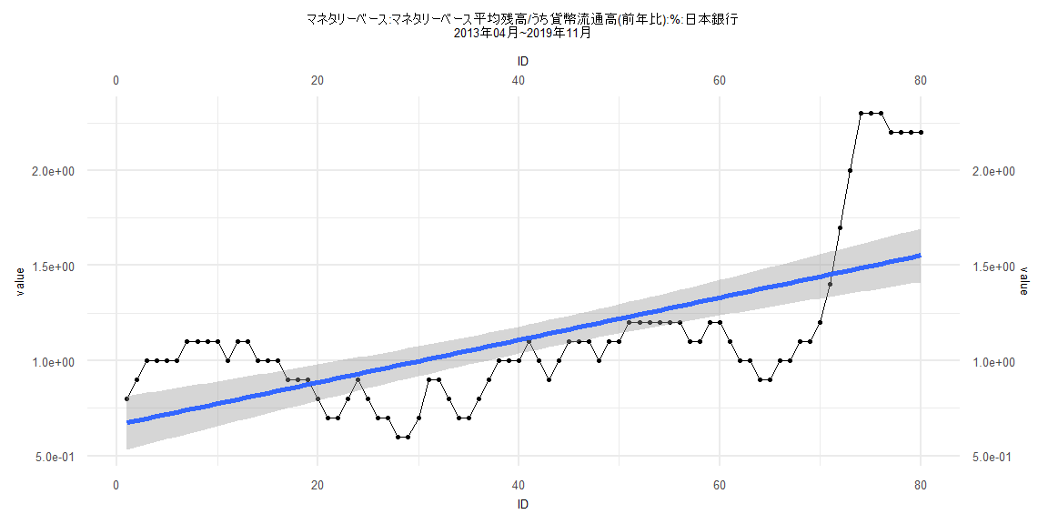
[1] "マネタリーベース:マネタリーベース平均残高/うち貨幣流通高(前年比):%:日本銀行"
      Jan  Feb  Mar  Apr  May  Jun  Jul  Aug  Sep  Oct  Nov  Dec
2000  1.6  1.6  1.4  1.3  1.1  1.1  1.0  1.9  1.8  1.6  1.4  0.9
2001  0.9  1.2  1.4  1.5  1.6  1.7  1.9  1.0  1.0  1.2  1.3  1.6
2002  1.7  1.6  1.5  1.6  1.9  2.0  2.0  2.0  2.1  2.1  2.1  1.9
2003  1.7  1.9  2.0  1.7  1.2  1.2  1.3  1.3  1.4  1.4  1.4  1.4
2004  1.3  1.4  1.5  1.5  1.7  1.9  1.9  1.9  1.9  2.0  1.9  1.7
2005  1.6  1.9  2.0  1.9  1.6  1.2  0.8  0.6  0.5  0.4  0.4  0.3
2006  0.3  0.1  0.0  0.2  0.4  0.6  0.7  0.8  0.8  0.8  0.7  0.6
2007  0.7  0.8  0.9  0.8  0.7  0.7  0.7  0.7  0.8  0.9  0.9  1.0
2008  1.0  1.0  1.0  0.9  0.8  0.8  0.8  0.7  0.7  0.6  0.5  0.4
2009  0.2  0.1 -0.1 -0.2 -0.2 -0.2 -0.2 -0.2 -0.1 -0.2 -0.4 -0.7
2010 -0.7 -0.7 -0.6 -0.5 -0.4 -0.3 -0.4 -0.3 -0.4 -0.5 -0.4 -0.4
2011 -0.2 -0.1  0.0  0.1  0.1  0.0  0.0  0.0  0.0  0.0  0.0  0.2
2012  0.1  0.1  0.1 -0.1 -0.1  0.0  0.2  0.3  0.4  0.4  0.4  0.5
2013  0.6  0.7  0.7  0.8  0.9  1.0  1.0  1.0  1.0  1.1  1.1  1.1
2014  1.1  1.0  1.1  1.1  1.0  1.0  1.0  0.9  0.9  0.9  0.8  0.7
2015  0.7  0.8  0.9  0.8  0.7  0.7  0.6  0.6  0.7  0.9  0.9  0.8
2016  0.7  0.7  0.8  0.9  1.0  1.0  1.0  1.1  1.0  0.9  1.0  1.1
2017  1.1  1.1  1.0  1.1  1.1  1.2  1.2  1.2  1.2  1.2  1.2  1.1
2018  1.1  1.2  1.2  1.1  1.0  1.0  0.9  0.9  1.0  1.0  1.1  1.1
2019  1.2  1.4  1.7  2.0  2.3  2.3  2.3  2.2  2.2  2.2  2.2
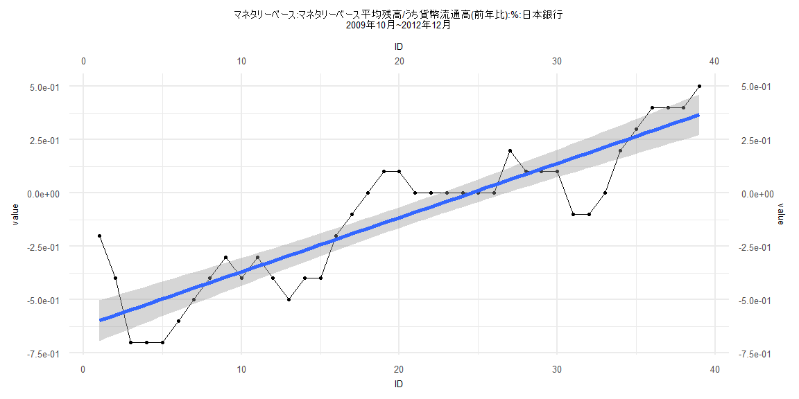
Call:
lm(formula = value ~ ID)

Residuals:
     Min       1Q   Median       3Q      Max
-0.28923 -0.10538  0.01385  0.09077  0.39769

Coefficients:
             Estimate Std. Error t value            Pr(>|t|)
(Intercept) -0.623077   0.048831  -12.76 0.00000000000000405 ***
ID           0.025385   0.002128   11.93 0.00000000000003031 ***
---
Signif. codes:  0 '***' 0.001 '**' 0.01 '*' 0.05 '.' 0.1 ' ' 1

Residual standard error: 0.1496 on 37 degrees of freedom
Multiple R-squared:  0.7937,    Adjusted R-squared:  0.7881
F-statistic: 142.3 on 1 and 37 DF,  p-value: 0.00000000000003031


    Two-sample Kolmogorov-Smirnov test

data:  lm_residuals and rnorm(n = length(lm_residuals), mean = 0, sd = sd(lm_residuals))
D = 0.12821, p-value = 0.9114
alternative hypothesis: two-sided


    Durbin-Watson test

data:  value ~ ID
DW = 0.55459, p-value = 0.00000000944
alternative hypothesis: true autocorrelation is greater than 0


    studentized Breusch-Pagan test

data:  value ~ ID
BP = 1.8362, df = 1, p-value = 0.1754


    Box-Ljung test

data:  lm_residuals
X-squared = 15.99, df = 1, p-value = 0.00006368
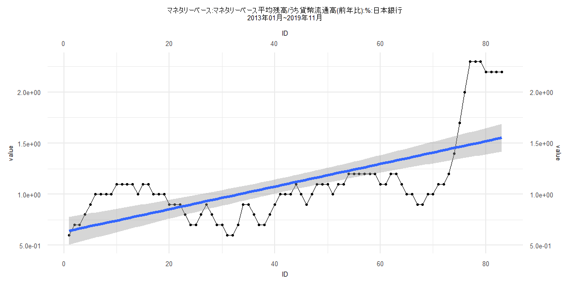
Call:
lm(formula = value ~ ID)

Residuals:
     Min       1Q   Median       3Q      Max
-0.48639 -0.20870 -0.08642  0.19675  0.81364

Coefficients:
            Estimate Std. Error t value           Pr(>|t|)
(Intercept) 0.631061   0.069538   9.075 0.0000000000000564 ***
ID          0.011108   0.001438   7.724 0.0000000000262318 ***
---
Signif. codes:  0 '***' 0.001 '**' 0.01 '*' 0.05 '.' 0.1 ' ' 1

Residual standard error: 0.3139 on 81 degrees of freedom
Multiple R-squared:  0.4241,    Adjusted R-squared:  0.417
F-statistic: 59.66 on 1 and 81 DF,  p-value: 0.00000000002623


    Two-sample Kolmogorov-Smirnov test

data:  lm_residuals and rnorm(n = length(lm_residuals), mean = 0, sd = sd(lm_residuals))
D = 0.14458, p-value = 0.3526
alternative hypothesis: two-sided


    Durbin-Watson test

data:  value ~ ID
DW = 0.089531, p-value < 0.00000000000000022
alternative hypothesis: true autocorrelation is greater than 0


    studentized Breusch-Pagan test

data:  value ~ ID
BP = 20.531, df = 1, p-value = 0.000005868


    Box-Ljung test

data:  lm_residuals
X-squared = 74.237, df = 1, p-value < 0.00000000000000022
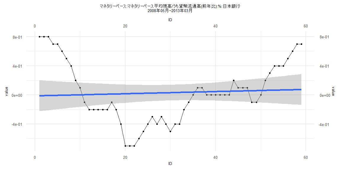
Call:
lm(formula = value ~ ID)

Residuals:
     Min       1Q   Median       3Q      Max
-0.72033 -0.22552 -0.04853  0.28291  0.81085

Coefficients:
             Estimate Std. Error t value Pr(>|t|)
(Intercept) -0.012332   0.108854  -0.113     0.91
ID           0.001485   0.003156   0.470     0.64

Residual standard error: 0.4128 on 57 degrees of freedom
Multiple R-squared:  0.003868,  Adjusted R-squared:  -0.01361
F-statistic: 0.2213 on 1 and 57 DF,  p-value: 0.6398


    Two-sample Kolmogorov-Smirnov test

data:  lm_residuals and rnorm(n = length(lm_residuals), mean = 0, sd = sd(lm_residuals))
D = 0.10169, p-value = 0.9239
alternative hypothesis: two-sided


    Durbin-Watson test

data:  value ~ ID
DW = 0.066977, p-value < 0.00000000000000022
alternative hypothesis: true autocorrelation is greater than 0


    studentized Breusch-Pagan test

data:  value ~ ID
BP = 9.9199, df = 1, p-value = 0.001635


    Box-Ljung test

data:  lm_residuals
X-squared = 51.675, df = 1, p-value = 0.0000000000006549
Call:
lm(formula = value ~ ID)

Residuals:
     Min       1Q   Median       3Q      Max
-0.48680 -0.21413 -0.08604  0.21511  0.81289

Coefficients:
            Estimate Std. Error t value          Pr(>|t|)
(Intercept) 0.662373   0.072179   9.177 0.000000000000049 ***
ID          0.011145   0.001548   7.199 0.000000000329150 ***
---
Signif. codes:  0 '***' 0.001 '**' 0.01 '*' 0.05 '.' 0.1 ' ' 1

Residual standard error: 0.3198 on 78 degrees of freedom
Multiple R-squared:  0.3992,    Adjusted R-squared:  0.3915
F-statistic: 51.82 on 1 and 78 DF,  p-value: 0.0000000003291


    Two-sample Kolmogorov-Smirnov test

data:  lm_residuals and rnorm(n = length(lm_residuals), mean = 0, sd = sd(lm_residuals))
D = 0.25, p-value = 0.01319
alternative hypothesis: two-sided


    Durbin-Watson test

data:  value ~ ID
DW = 0.087589, p-value < 0.00000000000000022
alternative hypothesis: true autocorrelation is greater than 0


    studentized Breusch-Pagan test

data:  value ~ ID
BP = 18.843, df = 1, p-value = 0.00001419


    Box-Ljung test

data:  lm_residuals
X-squared = 71.671, df = 1, p-value < 0.00000000000000022