Analysis
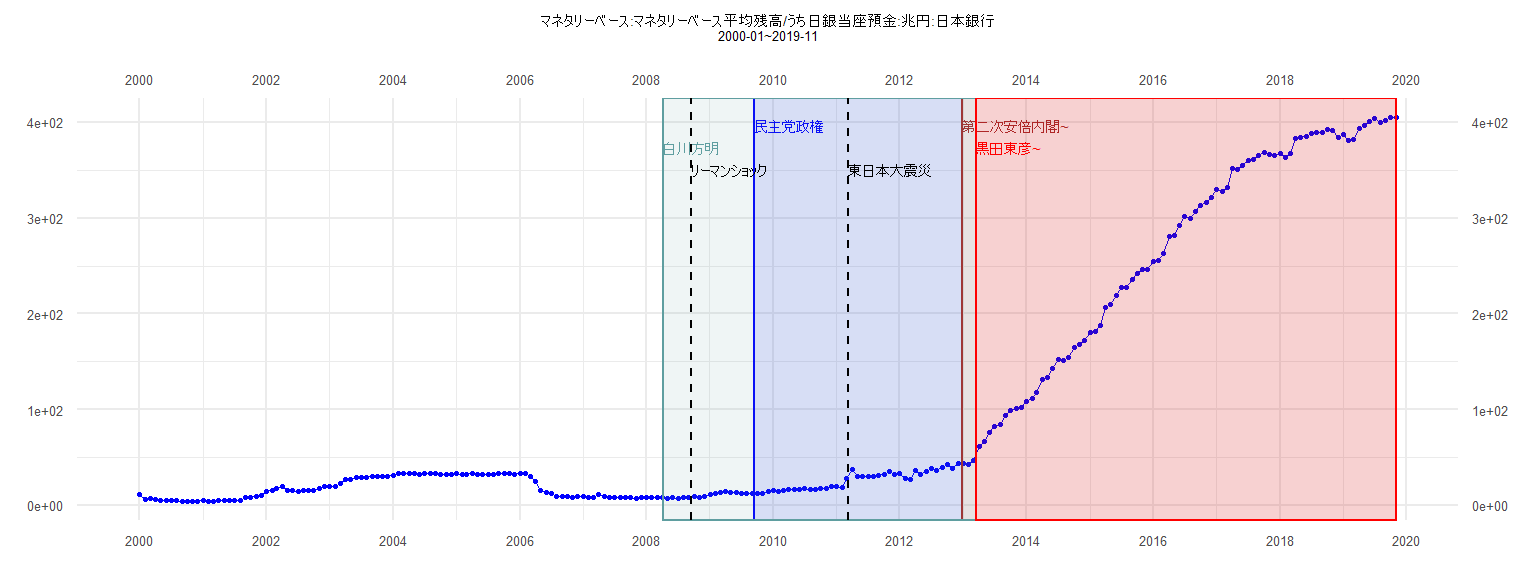
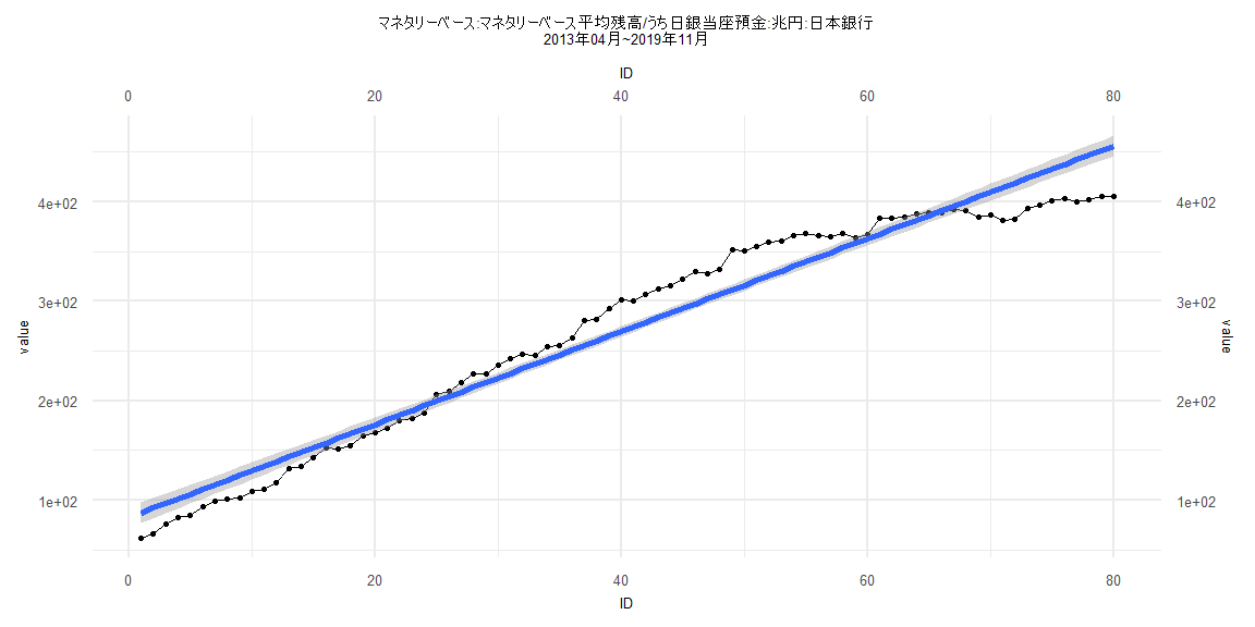
[1] "マネタリーベース:マネタリーベース平均残高/うち日銀当座預金:兆円:日本銀行"
          Jan      Feb      Mar      Apr      May      Jun      Jul      Aug      Sep      Oct      Nov      Dec
2000  11.4035   5.6760   6.7932   6.3286   5.2207   5.0879   5.3323   4.7265   3.9710   3.8232   3.8897   4.2036
2001   4.9913   4.2336   4.5394   5.0885   5.0757   5.0821   5.1016   5.5642   8.0824   8.5540   9.2093  10.8051
2002  14.9865  15.0328  17.5518  19.9864  15.6612  15.0415  14.9491  15.1299  15.2045  15.2212  18.0940  19.7901
2003  20.1250  20.0858  22.8332  27.4157  27.0292  28.8500  28.9139  29.2585  29.6788  29.7070  30.0204  29.9718
2004  31.2033  33.1991  33.0488  33.0181  33.2104  32.6309  32.9679  33.1496  32.9292  32.4975  32.5099  32.6367
2005  33.4166  32.6784  32.5719  33.0324  32.7343  31.9601  32.0817  32.1237  32.9000  33.4937  33.3352  32.2486
2006  33.6289  33.0879  30.4396  24.7613  15.1672  13.5173  11.9884   9.0511   8.7854   9.1240   7.8599   9.2552
2007   9.0102   8.5799   8.5517  11.0903   8.8833   8.4826   8.6870   8.6757   8.2780   8.2631   7.4838   8.2224
2008   7.7152   7.7834   7.9222   8.0654   7.4649   8.2960   7.6150   7.8009   8.7262   8.8459   8.3274   9.4319
2009  10.9378  12.9083  13.3936  14.6111  13.5616  13.2382  12.4288  12.8370  11.9996  12.7196  11.9375  14.4903
2010  15.6860  14.8834  15.1287  16.7404  16.6680  16.1079  17.3788  17.0379  16.6128  17.5564  17.5848  19.7892
2011  19.5315  18.3568  28.5498  37.4003  30.4210  30.4710  30.1126  30.5702  30.7103  32.4157  35.0151  31.9111
2012  33.1728  28.0484  27.5106  36.3191  31.8611  35.5032  38.0501  36.0747  39.1947  42.8428  38.8277  43.5567
2013  43.5197  42.4196  47.3674  61.9433  66.3050  76.1590  82.3519  84.3254  93.7486  98.7576 101.1535 101.8478
2014 108.6710 111.2480 117.8882 131.4470 133.6433 143.0031 152.1889 151.2314 154.9156 164.6186 167.6452 172.6512
2015 180.5957 181.9484 188.2382 206.1602 209.7476 218.7786 227.5161 227.2613 236.1564 242.4597 246.5776 246.1375
2016 254.7249 255.8817 262.7502 280.5584 281.3656 292.8396 301.7768 300.0575 306.6602 312.7923 316.0874 321.8408
2017 330.4487 327.4851 332.0877 351.8542 351.2682 355.1751 359.9452 360.7896 365.8174 368.2270 366.3521 365.1425
2018 368.0235 363.5595 367.4066 383.3311 384.1615 384.8228 388.3878 388.9556 389.4618 392.1148 391.4601 384.4459
2019 386.9959 381.6276 382.1401 393.7713 397.1398 401.1631 403.6991 400.1821 401.8207 405.0807 405.3420
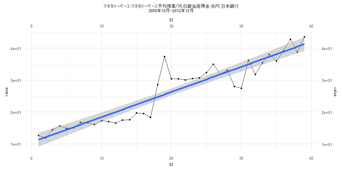
Call:
lm(formula = value ~ ID)

Residuals:
    Min      1Q  Median      3Q     Max
-6.6989 -2.1354  0.2556  1.9249 11.8617

Coefficients:
            Estimate Std. Error t value             Pr(>|t|)
(Intercept) 10.56160    1.11975   9.432       0.000000000022 ***
ID           0.78826    0.04879  16.155 < 0.0000000000000002 ***
---
Signif. codes:  0 '***' 0.001 '**' 0.01 '*' 0.05 '.' 0.1 ' ' 1

Residual standard error: 3.429 on 37 degrees of freedom
Multiple R-squared:  0.8758,    Adjusted R-squared:  0.8725
F-statistic:   261 on 1 and 37 DF,  p-value: < 0.00000000000000022


    Two-sample Kolmogorov-Smirnov test

data:  lm_residuals and rnorm(n = length(lm_residuals), mean = 0, sd = sd(lm_residuals))
D = 0.17949, p-value = 0.5622
alternative hypothesis: two-sided


    Durbin-Watson test

data:  value ~ ID
DW = 1.0518, p-value = 0.0003877
alternative hypothesis: true autocorrelation is greater than 0


    studentized Breusch-Pagan test

data:  value ~ ID
BP = 0.14807, df = 1, p-value = 0.7004


    Box-Ljung test

data:  lm_residuals
X-squared = 9.1429, df = 1, p-value = 0.002497
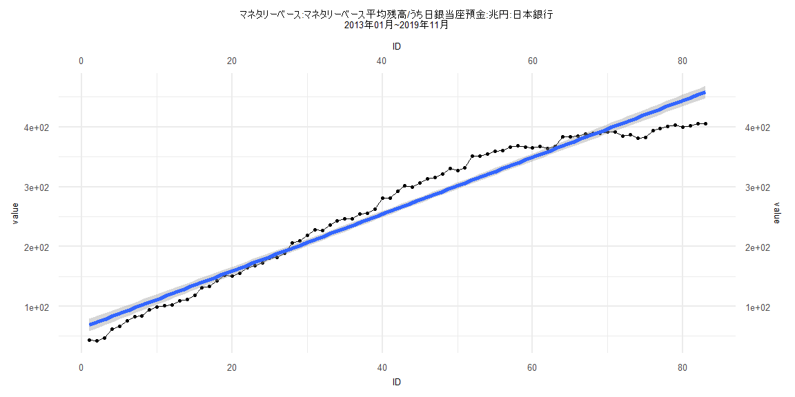
Call:
lm(formula = value ~ ID)

Residuals:
    Min      1Q  Median      3Q     Max
-53.323 -17.285  -2.151  16.475  40.597

Coefficients:
            Estimate Std. Error t value            Pr(>|t|)
(Intercept)  63.9929     5.2586   12.17 <0.0000000000000002 ***
ID            4.7551     0.1088   43.72 <0.0000000000000002 ***
---
Signif. codes:  0 '***' 0.001 '**' 0.01 '*' 0.05 '.' 0.1 ' ' 1

Residual standard error: 23.74 on 81 degrees of freedom
Multiple R-squared:  0.9594,    Adjusted R-squared:  0.9588
F-statistic:  1912 on 1 and 81 DF,  p-value: < 0.00000000000000022


    Two-sample Kolmogorov-Smirnov test

data:  lm_residuals and rnorm(n = length(lm_residuals), mean = 0, sd = sd(lm_residuals))
D = 0.084337, p-value = 0.9317
alternative hypothesis: two-sided


    Durbin-Watson test

data:  value ~ ID
DW = 0.04844, p-value < 0.00000000000000022
alternative hypothesis: true autocorrelation is greater than 0


    studentized Breusch-Pagan test

data:  value ~ ID
BP = 19.655, df = 1, p-value = 0.000009275


    Box-Ljung test

data:  lm_residuals
X-squared = 75.644, df = 1, p-value < 0.00000000000000022
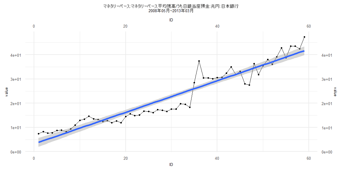
Call:
lm(formula = value ~ ID)

Residuals:
    Min      1Q  Median      3Q     Max
-7.0064 -2.7381  0.7809  2.3770 10.7325

Coefficients:
            Estimate Std. Error t value            Pr(>|t|)
(Intercept)  3.18433    0.92629   3.438              0.0011 **
ID           0.65232    0.02685  24.293 <0.0000000000000002 ***
---
Signif. codes:  0 '***' 0.001 '**' 0.01 '*' 0.05 '.' 0.1 ' ' 1

Residual standard error: 3.512 on 57 degrees of freedom
Multiple R-squared:  0.9119,    Adjusted R-squared:  0.9104
F-statistic: 590.2 on 1 and 57 DF,  p-value: < 0.00000000000000022


    Two-sample Kolmogorov-Smirnov test

data:  lm_residuals and rnorm(n = length(lm_residuals), mean = 0, sd = sd(lm_residuals))
D = 0.13559, p-value = 0.6544
alternative hypothesis: two-sided


    Durbin-Watson test

data:  value ~ ID
DW = 0.70486, p-value = 0.000000002539
alternative hypothesis: true autocorrelation is greater than 0


    studentized Breusch-Pagan test

data:  value ~ ID
BP = 1.0604, df = 1, p-value = 0.3031


    Box-Ljung test

data:  lm_residuals
X-squared = 23.48, df = 1, p-value = 0.000001262
Call:
lm(formula = value ~ ID)

Residuals:
    Min      1Q  Median      3Q     Max
-51.068 -19.478   3.503  17.392  40.227

Coefficients:
            Estimate Std. Error t value            Pr(>|t|)
(Intercept)  82.7785     5.2803   15.68 <0.0000000000000002 ***
ID            4.6704     0.1133   41.23 <0.0000000000000002 ***
---
Signif. codes:  0 '***' 0.001 '**' 0.01 '*' 0.05 '.' 0.1 ' ' 1

Residual standard error: 23.39 on 78 degrees of freedom
Multiple R-squared:  0.9561,    Adjusted R-squared:  0.9556
F-statistic:  1700 on 1 and 78 DF,  p-value: < 0.00000000000000022


    Two-sample Kolmogorov-Smirnov test

data:  lm_residuals and rnorm(n = length(lm_residuals), mean = 0, sd = sd(lm_residuals))
D = 0.1, p-value = 0.8219
alternative hypothesis: two-sided


    Durbin-Watson test

data:  value ~ ID
DW = 0.048618, p-value < 0.00000000000000022
alternative hypothesis: true autocorrelation is greater than 0


    studentized Breusch-Pagan test

data:  value ~ ID
BP = 18.244, df = 1, p-value = 0.00001943


    Box-Ljung test

data:  lm_residuals
X-squared = 72.986, df = 1, p-value < 0.00000000000000022