Analysis
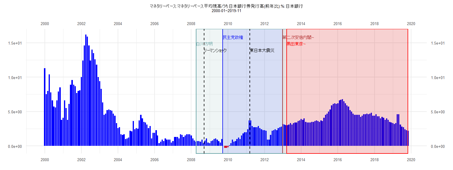
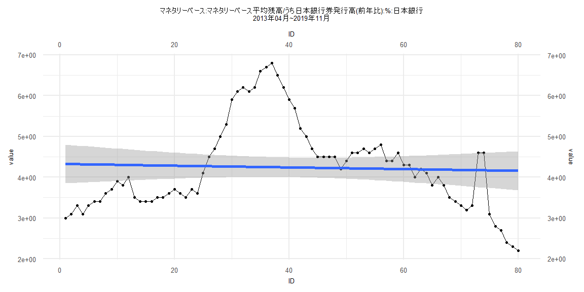
[1] "マネタリーベース:マネタリーベース平均残高/うち日本銀行券発行高(前年比):%:日本銀行"
      Jan  Feb  Mar  Apr  May  Jun  Jul  Aug  Sep  Oct  Nov  Dec
2000 11.3  7.5  8.0 10.4  7.8  6.6  5.7  5.6  6.6  7.9  8.5  3.8
2001  4.1  6.6  5.5  3.8  6.1  8.9  9.6  8.9  8.7  7.7  8.0  8.1
2002 10.0 12.4 14.6 16.2 15.9 14.6 12.4 14.0 13.5 12.6 11.8 10.0
2003  9.4  8.3  6.3  4.5  4.7  5.2  5.3  5.2  5.1  4.7  4.4  3.3
2004  2.6  2.7  1.7  1.6  1.7  1.0  1.1  1.2  2.2  2.1  3.6  2.4
2005  2.6  2.5  3.7  4.5  4.0  3.5  3.4  3.1  2.6  2.9  1.1  1.9
2006  1.9  2.3  1.5  0.4  0.6  0.9  0.7  1.1  0.9  0.9  0.9  0.5
2007  0.7  1.3  1.3  1.3  1.1  1.7  1.6  1.3  1.5  1.7  1.7  1.7
2008  1.5  1.1  0.8  0.6  0.7  0.7  0.6  0.9  0.4  0.8  1.1  0.5
2009  0.4  0.7  0.8  1.0  1.1  0.9  0.7  0.5  1.0  0.0 -0.3 -0.3
2010 -0.2  0.1  0.4  0.9  0.6  0.7  1.0  1.2  1.0  1.5  1.8  2.0
2011  2.0  2.4  3.7  3.7  2.9  2.7  2.7  2.7  2.9  2.6  2.4  2.3
2012  2.3  2.2  0.9  0.9  1.6  2.2  2.3  2.4  2.3  2.6  2.7  2.8
2013  3.2  3.1  3.0  3.0  3.1  3.3  3.1  3.3  3.4  3.4  3.6  3.7
2014  3.9  3.8  4.0  3.5  3.4  3.4  3.4  3.5  3.5  3.6  3.7  3.6
2015  3.5  3.7  3.6  4.1  4.5  4.7  5.0  5.3  5.9  6.1  6.2  6.1
2016  6.2  6.6  6.7  6.8  6.5  6.2  5.9  5.7  5.2  5.0  4.7  4.5
2017  4.5  4.5  4.5  4.2  4.4  4.6  4.6  4.7  4.6  4.7  4.8  4.4
2018  4.4  4.6  4.3  4.3  4.0  4.2  4.1  3.8  4.0  3.8  3.5  3.4
2019  3.3  3.2  3.3  4.6  4.6  3.1  2.8  2.7  2.4  2.3  2.2
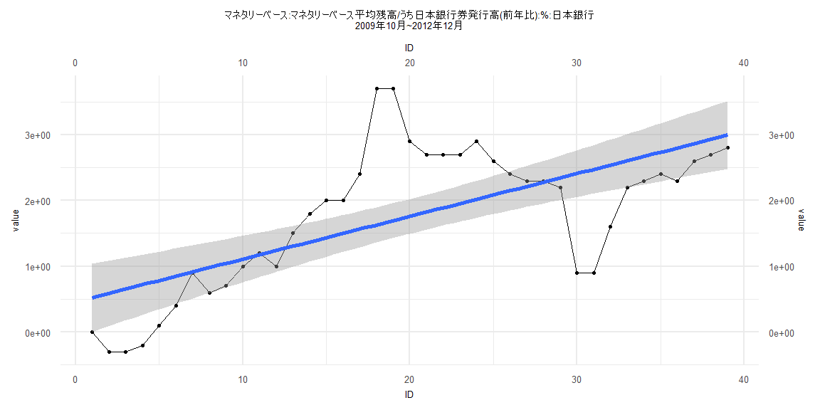
Call:
lm(formula = value ~ ID)

Residuals:
    Min      1Q  Median      3Q     Max
-1.5733 -0.4265 -0.1434  0.5086  2.0709

Coefficients:
            Estimate Std. Error t value   Pr(>|t|)
(Intercept)  0.46019    0.26571   1.732     0.0916 .
ID           0.06494    0.01158   5.609 0.00000213 ***
---
Signif. codes:  0 '***' 0.001 '**' 0.01 '*' 0.05 '.' 0.1 ' ' 1

Residual standard error: 0.8138 on 37 degrees of freedom
Multiple R-squared:  0.4595,    Adjusted R-squared:  0.4449
F-statistic: 31.46 on 1 and 37 DF,  p-value: 0.000002127


    Two-sample Kolmogorov-Smirnov test

data:  lm_residuals and rnorm(n = length(lm_residuals), mean = 0, sd = sd(lm_residuals))
D = 0.15385, p-value = 0.7523
alternative hypothesis: two-sided


    Durbin-Watson test

data:  value ~ ID
DW = 0.26025, p-value = 0.000000000000004418
alternative hypothesis: true autocorrelation is greater than 0


    studentized Breusch-Pagan test

data:  value ~ ID
BP = 0.00024804, df = 1, p-value = 0.9874


    Box-Ljung test

data:  lm_residuals
X-squared = 31.375, df = 1, p-value = 0.00000002127
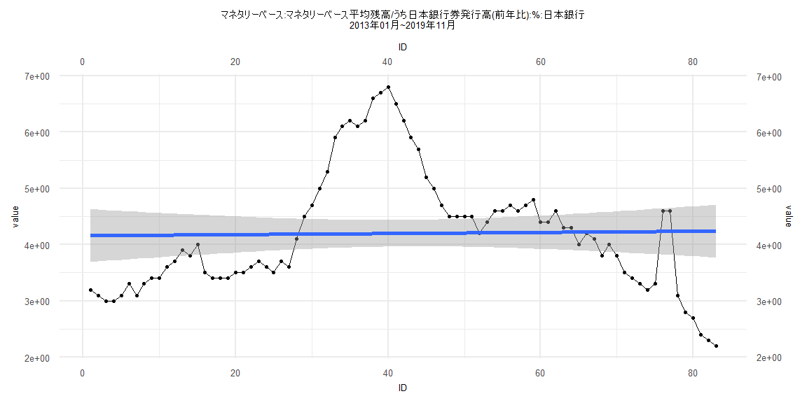
Call:
lm(formula = value ~ ID)

Residuals:
    Min      1Q  Median      3Q     Max
-2.0407 -0.7717 -0.1732  0.4361  2.6020

Coefficients:
             Estimate Std. Error t value            Pr(>|t|)
(Intercept) 4.1583015  0.2397486   17.34 <0.0000000000000002 ***
ID          0.0009928  0.0049583    0.20               0.842
---
Signif. codes:  0 '***' 0.001 '**' 0.01 '*' 0.05 '.' 0.1 ' ' 1

Residual standard error: 1.082 on 81 degrees of freedom
Multiple R-squared:  0.0004947, Adjusted R-squared:  -0.01184
F-statistic: 0.04009 on 1 and 81 DF,  p-value: 0.8418


    Two-sample Kolmogorov-Smirnov test

data:  lm_residuals and rnorm(n = length(lm_residuals), mean = 0, sd = sd(lm_residuals))
D = 0.14458, p-value = 0.3526
alternative hypothesis: two-sided


    Durbin-Watson test

data:  value ~ ID
DW = 0.081394, p-value < 0.00000000000000022
alternative hypothesis: true autocorrelation is greater than 0


    studentized Breusch-Pagan test

data:  value ~ ID
BP = 0.19229, df = 1, p-value = 0.661


    Box-Ljung test

data:  lm_residuals
X-squared = 74.815, df = 1, p-value < 0.00000000000000022
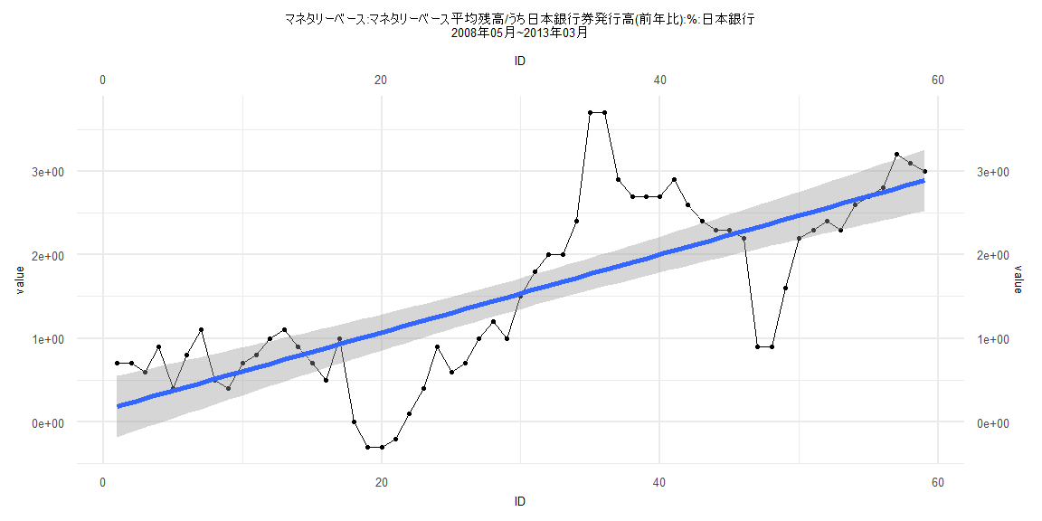
Call:
lm(formula = value ~ ID)

Residuals:
    Min      1Q  Median      3Q     Max
-1.4757 -0.3332  0.0640  0.3751  1.9298

Coefficients:
            Estimate Std. Error t value         Pr(>|t|)
(Intercept)  0.13986    0.18731   0.747            0.458
ID           0.04658    0.00543   8.579 0.00000000000758 ***
---
Signif. codes:  0 '***' 0.001 '**' 0.01 '*' 0.05 '.' 0.1 ' ' 1

Residual standard error: 0.7102 on 57 degrees of freedom
Multiple R-squared:  0.5635,    Adjusted R-squared:  0.5559
F-statistic:  73.6 on 1 and 57 DF,  p-value: 0.000000000007576


    Two-sample Kolmogorov-Smirnov test

data:  lm_residuals and rnorm(n = length(lm_residuals), mean = 0, sd = sd(lm_residuals))
D = 0.13559, p-value = 0.6544
alternative hypothesis: two-sided


    Durbin-Watson test

data:  value ~ ID
DW = 0.31863, p-value < 0.00000000000000022
alternative hypothesis: true autocorrelation is greater than 0


    studentized Breusch-Pagan test

data:  value ~ ID
BP = 0.18887, df = 1, p-value = 0.6639


    Box-Ljung test

data:  lm_residuals
X-squared = 43.355, df = 1, p-value = 0.00000000004565
Call:
lm(formula = value ~ ID)

Residuals:
    Min      1Q  Median      3Q     Max
-1.9584 -0.7926 -0.1329  0.4394  2.5514

Coefficients:
             Estimate Std. Error t value            Pr(>|t|)
(Intercept)  4.326171   0.243733  17.750 <0.0000000000000002 ***
ID          -0.002097   0.005228  -0.401               0.689
---
Signif. codes:  0 '***' 0.001 '**' 0.01 '*' 0.05 '.' 0.1 ' ' 1

Residual standard error: 1.08 on 78 degrees of freedom
Multiple R-squared:  0.002058,  Adjusted R-squared:  -0.01074
F-statistic: 0.1609 on 1 and 78 DF,  p-value: 0.6895


    Two-sample Kolmogorov-Smirnov test

data:  lm_residuals and rnorm(n = length(lm_residuals), mean = 0, sd = sd(lm_residuals))
D = 0.1125, p-value = 0.6953
alternative hypothesis: two-sided


    Durbin-Watson test

data:  value ~ ID
DW = 0.084632, p-value < 0.00000000000000022
alternative hypothesis: true autocorrelation is greater than 0


    studentized Breusch-Pagan test

data:  value ~ ID
BP = 0.014471, df = 1, p-value = 0.9042


    Box-Ljung test

data:  lm_residuals
X-squared = 71.351, df = 1, p-value < 0.00000000000000022