Analysis
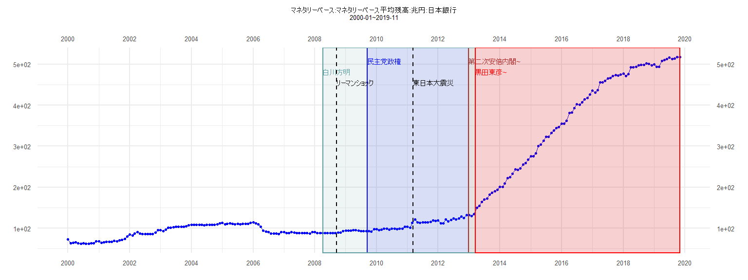
[1] "マネタリーベース:マネタリーベース平均残高:兆円:日本銀行"
          Jan      Feb      Mar      Apr      May      Jun      Jul      Aug      Sep      Oct      Nov      Dec
2000  72.1978  62.6865  64.9807  65.8350  63.7448  62.2152  63.7116  62.6193  61.8261  62.7618  63.5571  67.9588
2001  68.1280  64.7866  65.7361  66.7725  66.9654  66.9739  68.7826  68.2731  70.6356  71.7502  73.3778  79.4424
2002  84.0818  82.6163  87.1493  91.0393  86.8229  85.4332  86.0806  86.0881  85.7469  85.9299  89.4000  94.9444
2003  95.3668  93.0274  96.6459 101.5445 101.3547 102.7632 103.6363 103.7448 103.6332 103.6011 104.3362 107.4991
2004 108.3320 108.0570 108.1238 108.2958 108.8328 107.2957 108.5248 108.5653 108.5201 107.9234 109.4035 111.9769
2005 112.5134 109.3674 110.3301 111.5568 111.2725 109.1586 110.1137 109.7890 110.3950 110.9848 111.0432 113.0466
2006 114.1316 111.4431 109.2791 103.5779  94.1951  91.4229  90.5410  87.5607  86.9660  87.3279  86.2670  90.4664
2007  90.0507  87.9061  88.4022  90.8926  88.7868  87.6336  88.4708  88.1473  87.5728  87.7567  87.1633  90.7835
2008  89.9793  87.9916  88.3867  88.3589  87.9638  88.0155  87.8532  87.9433  88.3741  88.9825  88.8562  92.4351
2009  93.5049  93.6531  94.4658  95.6238  94.9165  93.6392  93.2096  93.3355  92.3942  92.8609  92.2042  97.2143
2010  98.0675  95.6928  96.4571  98.3836  98.4323  97.0240  98.9359  98.3995  97.7173  98.8248  99.1866 104.0238
2011 103.4826 101.0039 112.7432 121.8934 114.4208 113.4780 113.7324 114.0447 114.0181 115.6428 118.4978 118.0195
2012 118.9656 112.4409 112.4618 121.5003 117.1210 120.2142 123.5010 121.4626 124.3261 128.1344 124.4449 131.9837
2013 131.9205 129.3148 134.7413 149.5975 154.1412 163.5375 170.3890 172.4437 181.7012 186.8687 189.7244 193.4594
2014 200.4141 201.3223 208.5929 222.0795 224.3719 233.2465 243.1068 242.3138 245.8169 255.7542 259.3603 267.4016
2015 275.3859 275.2617 282.1182 300.3275 304.3476 313.0770 322.8211 322.9269 332.1941 338.8877 343.7218 346.3793
2016 355.1030 355.0415 362.6050 380.8364 381.8397 392.7119 402.4578 400.9981 407.5081 413.8966 417.6573 426.3922
2017 435.2054 430.9696 436.2634 456.2398 455.9954 459.4854 465.0692 466.3075 471.1205 473.8791 472.5834 474.1265
2018 477.2595 471.6382 475.9328 492.0203 492.9691 493.3638 497.6398 498.3868 498.8216 501.6198 501.3302 497.0034
2019 499.7797 493.0980 494.2027 507.3520 510.8086 512.9912 516.0145 512.5110 513.8266 517.1008 517.6305
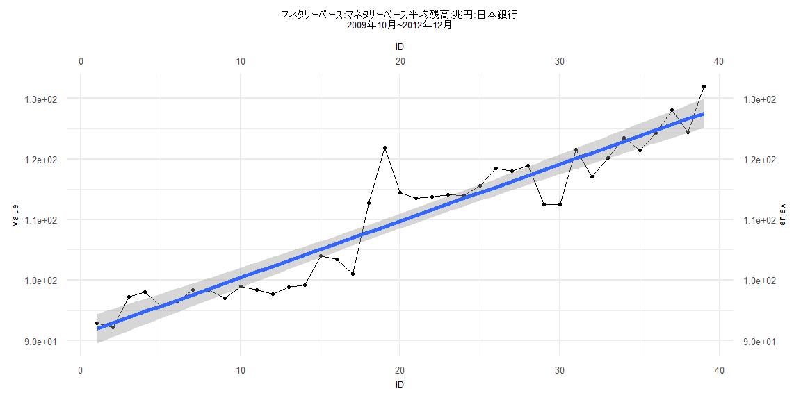
Call:
lm(formula = value ~ ID)

Residuals:
    Min      1Q  Median      3Q     Max
-6.6721 -2.3980 -0.0267  1.8980 13.0618

Coefficients:
            Estimate Std. Error t value            Pr(>|t|)
(Intercept) 91.03667    1.23556   73.68 <0.0000000000000002 ***
ID           0.93657    0.05384   17.40 <0.0000000000000002 ***
---
Signif. codes:  0 '***' 0.001 '**' 0.01 '*' 0.05 '.' 0.1 ' ' 1

Residual standard error: 3.784 on 37 degrees of freedom
Multiple R-squared:  0.8911,    Adjusted R-squared:  0.8881
F-statistic: 302.6 on 1 and 37 DF,  p-value: < 0.00000000000000022


    Two-sample Kolmogorov-Smirnov test

data:  lm_residuals and rnorm(n = length(lm_residuals), mean = 0, sd = sd(lm_residuals))
D = 0.10256, p-value = 0.9885
alternative hypothesis: two-sided


    Durbin-Watson test

data:  value ~ ID
DW = 1.1047, p-value = 0.000788
alternative hypothesis: true autocorrelation is greater than 0


    studentized Breusch-Pagan test

data:  value ~ ID
BP = 0.042383, df = 1, p-value = 0.8369


    Box-Ljung test

data:  lm_residuals
X-squared = 7.7244, df = 1, p-value = 0.005448
Call:
lm(formula = value ~ ID)

Residuals:
    Min      1Q  Median      3Q     Max
-55.732 -16.874  -1.714  17.477  41.224

Coefficients:
            Estimate Std. Error t value            Pr(>|t|)
(Intercept)  149.401      5.318   28.10 <0.0000000000000002 ***
ID             5.108      0.110   46.45 <0.0000000000000002 ***
---
Signif. codes:  0 '***' 0.001 '**' 0.01 '*' 0.05 '.' 0.1 ' ' 1

Residual standard error: 24 on 81 degrees of freedom
Multiple R-squared:  0.9638,    Adjusted R-squared:  0.9634
F-statistic:  2157 on 1 and 81 DF,  p-value: < 0.00000000000000022


    Two-sample Kolmogorov-Smirnov test

data:  lm_residuals and rnorm(n = length(lm_residuals), mean = 0, sd = sd(lm_residuals))
D = 0.072289, p-value = 0.9829
alternative hypothesis: two-sided


    Durbin-Watson test

data:  value ~ ID
DW = 0.049212, p-value < 0.00000000000000022
alternative hypothesis: true autocorrelation is greater than 0


    studentized Breusch-Pagan test

data:  value ~ ID
BP = 20.488, df = 1, p-value = 0.000006


    Box-Ljung test

data:  lm_residuals
X-squared = 75.481, df = 1, p-value < 0.00000000000000022
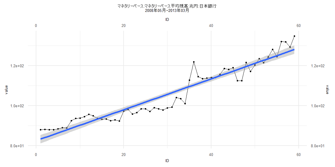
Call:
lm(formula = value ~ ID)

Residuals:
    Min      1Q  Median      3Q     Max
-7.7148 -3.2634  0.7444  2.9539 11.6298

Coefficients:
            Estimate Std. Error t value            Pr(>|t|)
(Intercept) 82.45486    1.08054   76.31 <0.0000000000000002 ***
ID           0.77247    0.03132   24.66 <0.0000000000000002 ***
---
Signif. codes:  0 '***' 0.001 '**' 0.01 '*' 0.05 '.' 0.1 ' ' 1

Residual standard error: 4.097 on 57 degrees of freedom
Multiple R-squared:  0.9143,    Adjusted R-squared:  0.9128
F-statistic: 608.2 on 1 and 57 DF,  p-value: < 0.00000000000000022


    Two-sample Kolmogorov-Smirnov test

data:  lm_residuals and rnorm(n = length(lm_residuals), mean = 0, sd = sd(lm_residuals))
D = 0.25424, p-value = 0.04374
alternative hypothesis: two-sided


    Durbin-Watson test

data:  value ~ ID
DW = 0.67286, p-value = 0.0000000007934
alternative hypothesis: true autocorrelation is greater than 0


    studentized Breusch-Pagan test

data:  value ~ ID
BP = 0.64799, df = 1, p-value = 0.4208


    Box-Ljung test

data:  lm_residuals
X-squared = 24.497, df = 1, p-value = 0.0000007444
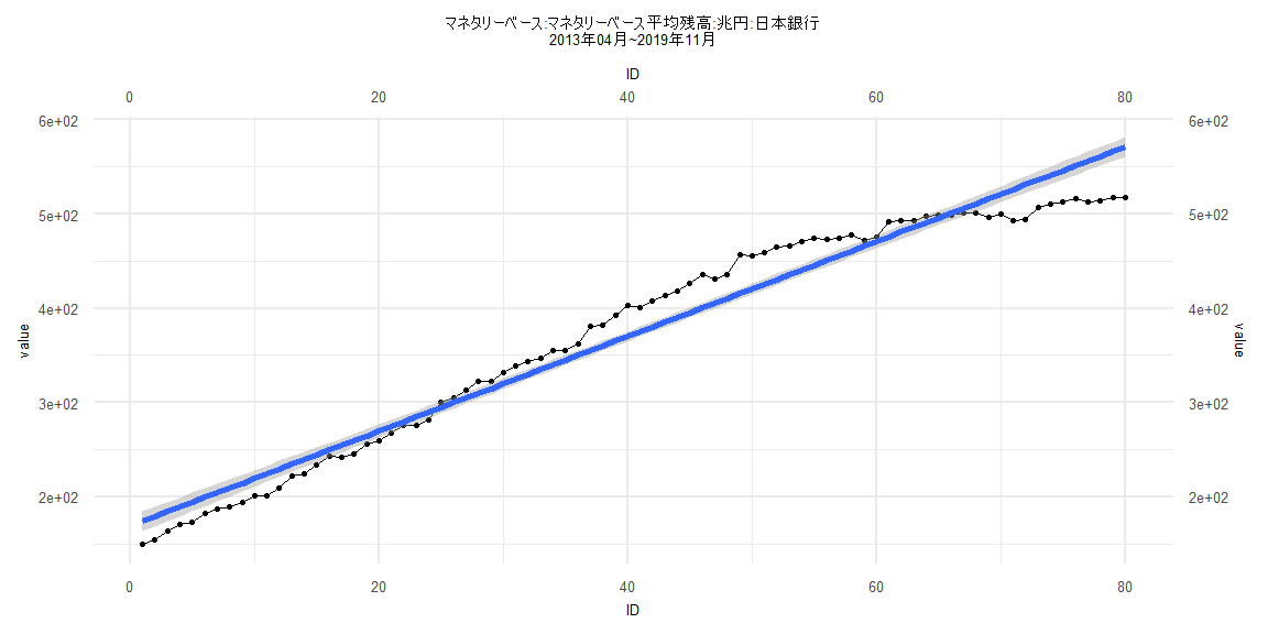
Call:
lm(formula = value ~ ID)

Residuals:
    Min      1Q  Median      3Q     Max
-53.590 -18.889   3.596  19.348  40.872

Coefficients:
            Estimate Std. Error t value            Pr(>|t|)
(Intercept)  169.019      5.360   31.53 <0.0000000000000002 ***
ID             5.027      0.115   43.73 <0.0000000000000002 ***
---
Signif. codes:  0 '***' 0.001 '**' 0.01 '*' 0.05 '.' 0.1 ' ' 1

Residual standard error: 23.75 on 78 degrees of freedom
Multiple R-squared:  0.9608,    Adjusted R-squared:  0.9603
F-statistic:  1912 on 1 and 78 DF,  p-value: < 0.00000000000000022


    Two-sample Kolmogorov-Smirnov test

data:  lm_residuals and rnorm(n = length(lm_residuals), mean = 0, sd = sd(lm_residuals))
D = 0.0875, p-value = 0.922
alternative hypothesis: two-sided


    Durbin-Watson test

data:  value ~ ID
DW = 0.048587, p-value < 0.00000000000000022
alternative hypothesis: true autocorrelation is greater than 0


    studentized Breusch-Pagan test

data:  value ~ ID
BP = 18.796, df = 1, p-value = 0.00001455


    Box-Ljung test

data:  lm_residuals
X-squared = 72.79, df = 1, p-value < 0.00000000000000022