Analysis
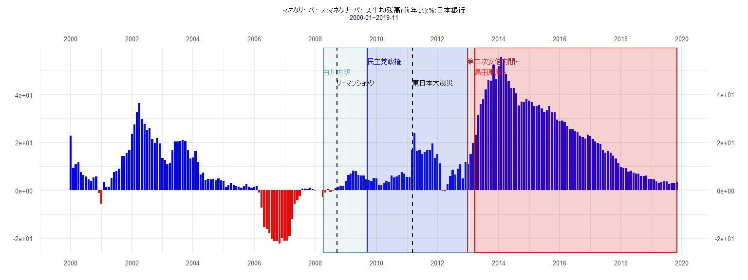
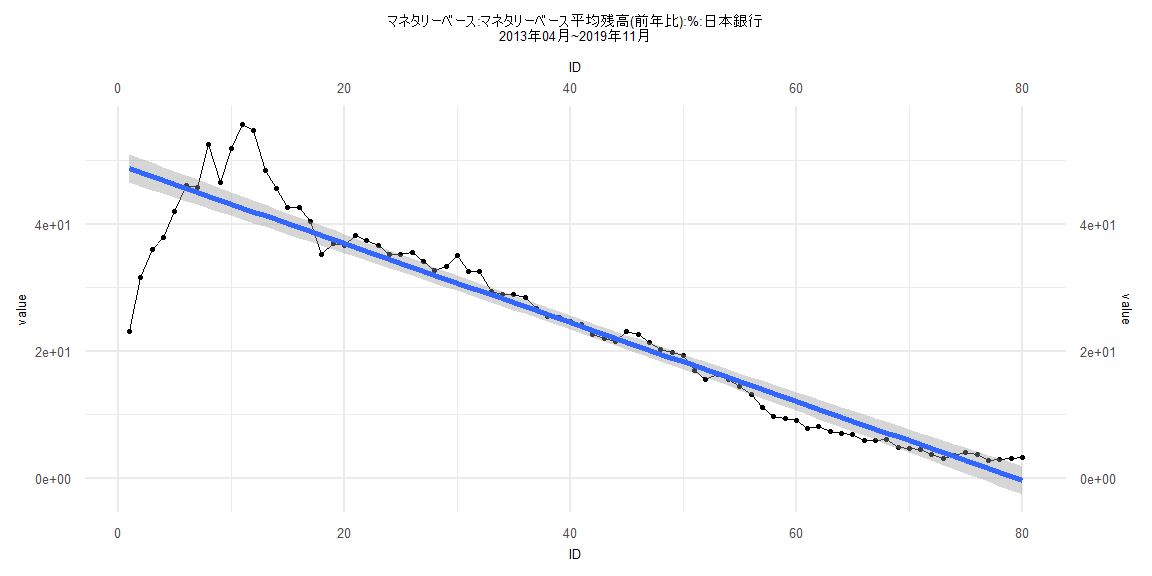
[1] "マネタリーベース:マネタリーベース平均残高(前年比):%:日本銀行"
       Jan   Feb   Mar   Apr   May   Jun   Jul   Aug   Sep   Oct   Nov   Dec
2000  22.8   9.4  10.9  11.7   7.6   6.4   5.8   4.6   4.0   5.3   5.7  -1.1
2001  -5.6   3.4   1.2   1.4   5.1   7.6   8.0   9.0  14.2  14.3  15.5  16.9
2002  23.4  27.5  32.6  36.3  29.7  27.6  25.1  26.1  21.4  19.8  21.8  19.5
2003  13.4  12.6  10.9  11.5  16.7  20.3  20.4  20.5  20.9  20.6  16.7  13.2
2004  13.6  16.2  11.9   6.6   7.4   4.4   4.7   4.6   4.7   4.2   4.9   4.2
2005   3.9   1.2   2.0   3.0   2.2   1.7   1.5   1.1   1.7   2.8   1.5   1.0
2006   1.4   1.9  -1.0  -7.2 -15.3 -16.2 -17.8 -20.2 -21.2 -21.3 -22.3 -20.0
2007 -21.1 -21.1 -19.1 -12.2  -5.7  -4.1  -2.3   0.7   0.7   0.5   1.0   0.4
2008  -0.1   0.1   0.0  -2.8  -0.9   0.4  -0.7  -0.2   0.9   1.4   1.9   1.8
2009   3.9   6.4   6.9   8.2   7.9   6.4   6.1   6.1   4.5   4.4   3.8   5.2
2010   4.9   2.2   2.1   2.9   3.7   3.6   6.1   5.4   5.8   6.4   7.6   7.0
2011   5.5   5.6  16.9  23.9  16.2  17.0  15.0  15.9  16.7  17.0  19.5  13.5
2012  15.0  11.3  -0.2  -0.3   2.4   5.9   8.6   6.5   9.0  10.8   5.0  11.8
2013  10.9  15.0  19.8  23.1  31.6  36.0  38.0  42.0  46.1  45.8  52.5  46.6
2014  51.9  55.7  54.8  48.5  45.6  42.6  42.7  40.5  35.3  36.9  36.7  38.2
2015  37.4  36.7  35.2  35.2  35.6  34.2  32.8  33.3  35.1  32.5  32.5  29.5
2016  28.9  29.0  28.5  26.8  25.5  25.4  24.7  24.2  22.7  22.1  21.5  23.1
2017  22.6  21.4  20.3  19.8  19.4  17.0  15.6  16.3  15.6  14.5  13.2  11.2
2018   9.7   9.4   9.1   7.8   8.1   7.4   7.0   6.9   5.9   5.9   6.1   4.8
2019   4.7   4.6   3.8   3.1   3.6   4.0   3.7   2.8   3.0   3.1   3.3
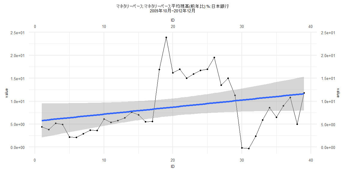
Call:
lm(formula = value ~ ID)

Residuals:
    Min      1Q  Median      3Q     Max
-10.697  -3.291  -1.350   4.390  15.346

Coefficients:
            Estimate Std. Error t value Pr(>|t|)
(Intercept)  5.63563    1.89992   2.966  0.00526 **
ID           0.15360    0.08279   1.855  0.07152 .
---
Signif. codes:  0 '***' 0.001 '**' 0.01 '*' 0.05 '.' 0.1 ' ' 1

Residual standard error: 5.819 on 37 degrees of freedom
Multiple R-squared:  0.08512,   Adjusted R-squared:  0.06039
F-statistic: 3.442 on 1 and 37 DF,  p-value: 0.07152


    Two-sample Kolmogorov-Smirnov test

data:  lm_residuals and rnorm(n = length(lm_residuals), mean = 0, sd = sd(lm_residuals))
D = 0.25641, p-value = 0.1547
alternative hypothesis: two-sided


    Durbin-Watson test

data:  value ~ ID
DW = 0.45832, p-value = 0.0000000002809
alternative hypothesis: true autocorrelation is greater than 0


    studentized Breusch-Pagan test

data:  value ~ ID
BP = 2.1261, df = 1, p-value = 0.1448


    Box-Ljung test

data:  lm_residuals
X-squared = 24.952, df = 1, p-value = 0.0000005877
Call:
lm(formula = value ~ ID)

Residuals:
    Min      1Q  Median      3Q     Max
-34.875  -2.581   1.064   3.862  16.860

Coefficients:
            Estimate Std. Error t value            Pr(>|t|)
(Intercept) 46.30817    1.76563   26.23 <0.0000000000000002 ***
ID          -0.53347    0.03652  -14.61 <0.0000000000000002 ***
---
Signif. codes:  0 '***' 0.001 '**' 0.01 '*' 0.05 '.' 0.1 ' ' 1

Residual standard error: 7.97 on 81 degrees of freedom
Multiple R-squared:  0.7249,    Adjusted R-squared:  0.7215
F-statistic: 213.4 on 1 and 81 DF,  p-value: < 0.00000000000000022


    Two-sample Kolmogorov-Smirnov test

data:  lm_residuals and rnorm(n = length(lm_residuals), mean = 0, sd = sd(lm_residuals))
D = 0.25301, p-value = 0.009606
alternative hypothesis: two-sided


    Durbin-Watson test

data:  value ~ ID
DW = 0.093015, p-value < 0.00000000000000022
alternative hypothesis: true autocorrelation is greater than 0


    studentized Breusch-Pagan test

data:  value ~ ID
BP = 17.305, df = 1, p-value = 0.00003184


    Box-Ljung test

data:  lm_residuals
X-squared = 60.009, df = 1, p-value = 0.000000000000009437
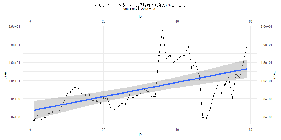
Call:
lm(formula = value ~ ID)

Residuals:
     Min       1Q   Median       3Q      Max
-11.4028  -2.7572  -0.9576   2.9188  15.1561

Coefficients:
            Estimate Std. Error t value   Pr(>|t|)
(Intercept)  1.66715    1.30948   1.273      0.208
ID           0.19658    0.03796   5.179 0.00000304 ***
---
Signif. codes:  0 '***' 0.001 '**' 0.01 '*' 0.05 '.' 0.1 ' ' 1

Residual standard error: 4.965 on 57 degrees of freedom
Multiple R-squared:  0.3199,    Adjusted R-squared:  0.308
F-statistic: 26.82 on 1 and 57 DF,  p-value: 0.000003038


    Two-sample Kolmogorov-Smirnov test

data:  lm_residuals and rnorm(n = length(lm_residuals), mean = 0, sd = sd(lm_residuals))
D = 0.22034, p-value = 0.1141
alternative hypothesis: two-sided


    Durbin-Watson test

data:  value ~ ID
DW = 0.45027, p-value = 0.00000000000002004
alternative hypothesis: true autocorrelation is greater than 0


    studentized Breusch-Pagan test

data:  value ~ ID
BP = 7.4667, df = 1, p-value = 0.006285


    Box-Ljung test

data:  lm_residuals
X-squared = 35.554, df = 1, p-value = 0.00000000248
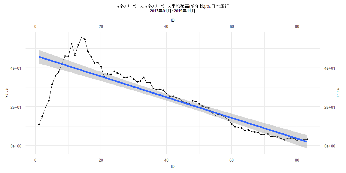
Call:
lm(formula = value ~ ID)

Residuals:
     Min       1Q   Median       3Q      Max
-25.6681  -1.2492   0.4182   1.6740  13.1447

Coefficients:
            Estimate Std. Error t value            Pr(>|t|)
(Intercept)  49.3893     1.1327   43.60 <0.0000000000000002 ***
ID           -0.6213     0.0243  -25.57 <0.0000000000000002 ***
---
Signif. codes:  0 '***' 0.001 '**' 0.01 '*' 0.05 '.' 0.1 ' ' 1

Residual standard error: 5.018 on 78 degrees of freedom
Multiple R-squared:  0.8934,    Adjusted R-squared:  0.8921
F-statistic: 653.9 on 1 and 78 DF,  p-value: < 0.00000000000000022


    Two-sample Kolmogorov-Smirnov test

data:  lm_residuals and rnorm(n = length(lm_residuals), mean = 0, sd = sd(lm_residuals))
D = 0.2, p-value = 0.08141
alternative hypothesis: two-sided


    Durbin-Watson test

data:  value ~ ID
DW = 0.21309, p-value < 0.00000000000000022
alternative hypothesis: true autocorrelation is greater than 0


    studentized Breusch-Pagan test

data:  value ~ ID
BP = 11.976, df = 1, p-value = 0.0005388


    Box-Ljung test

data:  lm_residuals
X-squared = 43.335, df = 1, p-value = 0.00000000004612