Analysis
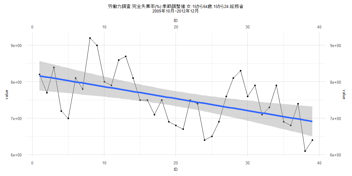
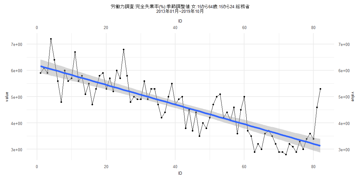
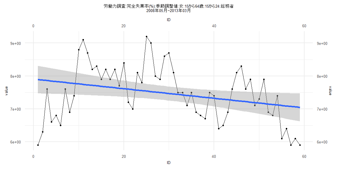
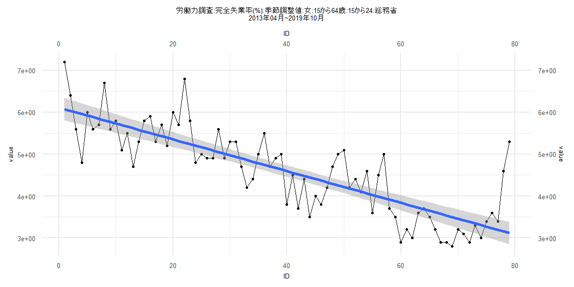
[1] "労働力調査:完全失業率(%):季節調整値:女:15から64歳:15から24:総務省"
     Jan Feb Mar Apr May Jun Jul Aug Sep Oct Nov Dec
1999                                             7.4
2000 7.2 7.6 7.7 7.6 7.7 8.0 7.5 7.5 8.0 7.9 9.0 9.2
2001 8.4 8.3 8.4 8.0 8.3 8.7 8.6 8.7 9.3 8.9 8.3 8.0
2002 8.5 8.8 8.8 8.7 9.1 9.3 9.0 9.1 8.3 8.0 7.0 8.8
2003 9.2 9.2 9.2 9.5 9.0 9.0 8.2 7.9 8.0 8.0 8.3 7.7
2004 9.0 8.0 8.4 8.1 8.1 7.4 8.2 8.2 7.4 8.1 8.4 7.7
2005 6.5 7.2 7.0 7.9 7.6 6.8 7.8 7.3 7.0 7.8 7.9 8.1
2006 6.9 6.1 7.0 7.2 7.2 8.5 7.3 6.6 7.3 7.2 6.4 6.3
2007 8.2 8.0 6.8 6.2 6.5 6.2 5.7 8.1 8.5 7.3 7.1 7.6
2008 6.7 7.0 6.3 6.5 5.9 6.3 7.6 6.6 6.8 6.5 7.6 6.9
2009 7.4 8.8 9.1 8.7 8.2 8.3 7.9 8.2 7.9 8.2 7.7 8.4
2010 7.2 7.0 8.1 7.8 9.2 9.0 8.0 7.9 8.6 8.7 8.1 7.5
2011 7.5 7.1 7.5 6.9 6.8 6.7 7.5 7.4 6.4 6.5 6.9 7.6
2012 8.1 8.3 7.6 7.9 7.1 7.3 7.9 6.9 6.8 7.4 6.1 6.4
2013 5.9 6.1 5.9 7.2 6.4 5.6 4.8 6.0 5.6 5.7 6.7 5.6
2014 5.8 5.1 5.5 4.7 5.3 5.8 5.9 5.3 5.7 5.2 6.0 5.7
2015 6.8 5.8 4.8 5.0 4.9 4.9 5.6 4.9 5.3 5.3 4.7 4.2
2016 4.4 5.0 5.5 4.7 4.9 5.0 3.8 4.5 3.7 4.4 3.5 4.0
2017 3.8 4.2 4.7 5.0 5.1 4.2 4.4 4.1 4.6 3.6 4.5 5.0
2018 3.7 3.5 2.9 3.2 3.0 3.6 3.7 3.5 3.2 2.9 2.9 2.8
2019 3.2 3.1 2.9 3.3 3.0 3.4 3.6 3.4 4.6 5.3
Call:
lm(formula = value ~ ID)

Residuals:
     Min       1Q   Median       3Q      Max
-1.03188 -0.47728 -0.03978  0.37733  1.26680

Coefficients:
             Estimate Std. Error t value             Pr(>|t|)
(Intercept)  8.196356   0.208499  39.311 < 0.0000000000000002 ***
ID          -0.032895   0.009085  -3.621             0.000875 ***
---
Signif. codes:  0 '***' 0.001 '**' 0.01 '*' 0.05 '.' 0.1 ' ' 1

Residual standard error: 0.6386 on 37 degrees of freedom
Multiple R-squared:  0.2616,    Adjusted R-squared:  0.2417
F-statistic: 13.11 on 1 and 37 DF,  p-value: 0.000875


    Two-sample Kolmogorov-Smirnov test

data:  lm_residuals and rnorm(n = length(lm_residuals), mean = 0, sd = sd(lm_residuals))
D = 0.12821, p-value = 0.9114
alternative hypothesis: two-sided


    Durbin-Watson test

data:  value ~ ID
DW = 1.0435, p-value = 0.0003452
alternative hypothesis: true autocorrelation is greater than 0


    studentized Breusch-Pagan test

data:  value ~ ID
BP = 0.25113, df = 1, p-value = 0.6163


    Box-Ljung test

data:  lm_residuals
X-squared = 9.2749, df = 1, p-value = 0.002323
Call:
lm(formula = value ~ ID)

Residuals:
    Min      1Q  Median      3Q     Max
-1.1376 -0.3780 -0.1268  0.3518  2.1695

Coefficients:
             Estimate Std. Error t value            Pr(>|t|)
(Intercept)  6.199639   0.132585   46.76 <0.0000000000000002 ***
ID          -0.037429   0.002775  -13.49 <0.0000000000000002 ***
---
Signif. codes:  0 '***' 0.001 '**' 0.01 '*' 0.05 '.' 0.1 ' ' 1

Residual standard error: 0.5948 on 80 degrees of freedom
Multiple R-squared:  0.6945,    Adjusted R-squared:  0.6907
F-statistic: 181.9 on 1 and 80 DF,  p-value: < 0.00000000000000022


    Two-sample Kolmogorov-Smirnov test

data:  lm_residuals and rnorm(n = length(lm_residuals), mean = 0, sd = sd(lm_residuals))
D = 0.10976, p-value = 0.7099
alternative hypothesis: two-sided


    Durbin-Watson test

data:  value ~ ID
DW = 1.0863, p-value = 0.000003159
alternative hypothesis: true autocorrelation is greater than 0


    studentized Breusch-Pagan test

data:  value ~ ID
BP = 2.1081, df = 1, p-value = 0.1465


    Box-Ljung test

data:  lm_residuals
X-squared = 11.798, df = 1, p-value = 0.000593
Call:
lm(formula = value ~ ID)

Residuals:
     Min       1Q   Median       3Q      Max
-1.99034 -0.57508  0.07791  0.54378  1.65935

Coefficients:
             Estimate Std. Error t value            Pr(>|t|)
(Intercept)  7.904909   0.215885  36.616 <0.0000000000000002 ***
ID          -0.014570   0.006258  -2.328              0.0235 *
---
Signif. codes:  0 '***' 0.001 '**' 0.01 '*' 0.05 '.' 0.1 ' ' 1

Residual standard error: 0.8186 on 57 degrees of freedom
Multiple R-squared:  0.08684,   Adjusted R-squared:  0.07082
F-statistic: 5.421 on 1 and 57 DF,  p-value: 0.02347


    Two-sample Kolmogorov-Smirnov test

data:  lm_residuals and rnorm(n = length(lm_residuals), mean = 0, sd = sd(lm_residuals))
D = 0.18644, p-value = 0.2582
alternative hypothesis: two-sided


    Durbin-Watson test

data:  value ~ ID
DW = 0.62813, p-value = 0.000000000138
alternative hypothesis: true autocorrelation is greater than 0


    studentized Breusch-Pagan test

data:  value ~ ID
BP = 4.5989, df = 1, p-value = 0.03199


    Box-Ljung test

data:  lm_residuals
X-squared = 23.615, df = 1, p-value = 0.000001176
Call:
lm(formula = value ~ ID)

Residuals:
    Min      1Q  Median      3Q     Max
-1.1607 -0.4007 -0.1244  0.3630  2.1821

Coefficients:
             Estimate Std. Error t value            Pr(>|t|)
(Intercept)  6.112366   0.137449   44.47 <0.0000000000000002 ***
ID          -0.037904   0.002985  -12.70 <0.0000000000000002 ***
---
Signif. codes:  0 '***' 0.001 '**' 0.01 '*' 0.05 '.' 0.1 ' ' 1

Residual standard error: 0.605 on 77 degrees of freedom
Multiple R-squared:  0.6768,    Adjusted R-squared:  0.6726
F-statistic: 161.2 on 1 and 77 DF,  p-value: < 0.00000000000000022


    Two-sample Kolmogorov-Smirnov test

data:  lm_residuals and rnorm(n = length(lm_residuals), mean = 0, sd = sd(lm_residuals))
D = 0.1519, p-value = 0.3233
alternative hypothesis: two-sided


    Durbin-Watson test

data:  value ~ ID
DW = 1.0245, p-value = 0.0000009116
alternative hypothesis: true autocorrelation is greater than 0


    studentized Breusch-Pagan test

data:  value ~ ID
BP = 1.5382, df = 1, p-value = 0.2149


    Box-Ljung test

data:  lm_residuals
X-squared = 11.899, df = 1, p-value = 0.0005617