Analysis
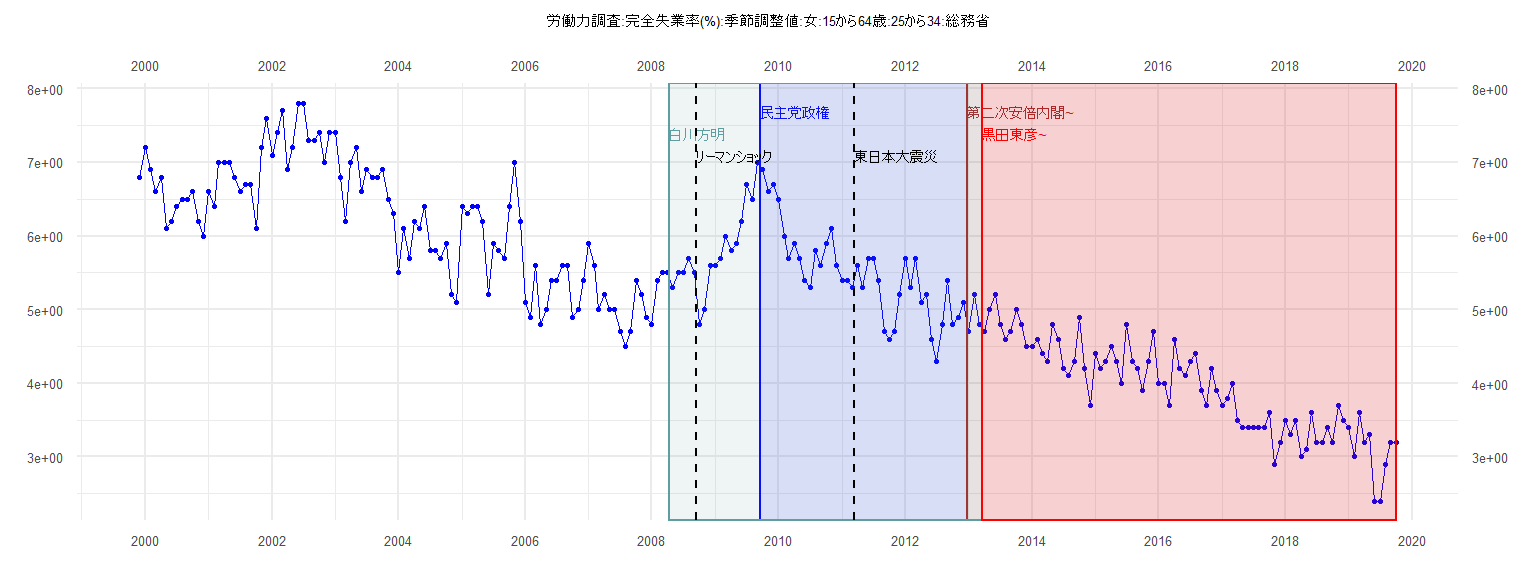
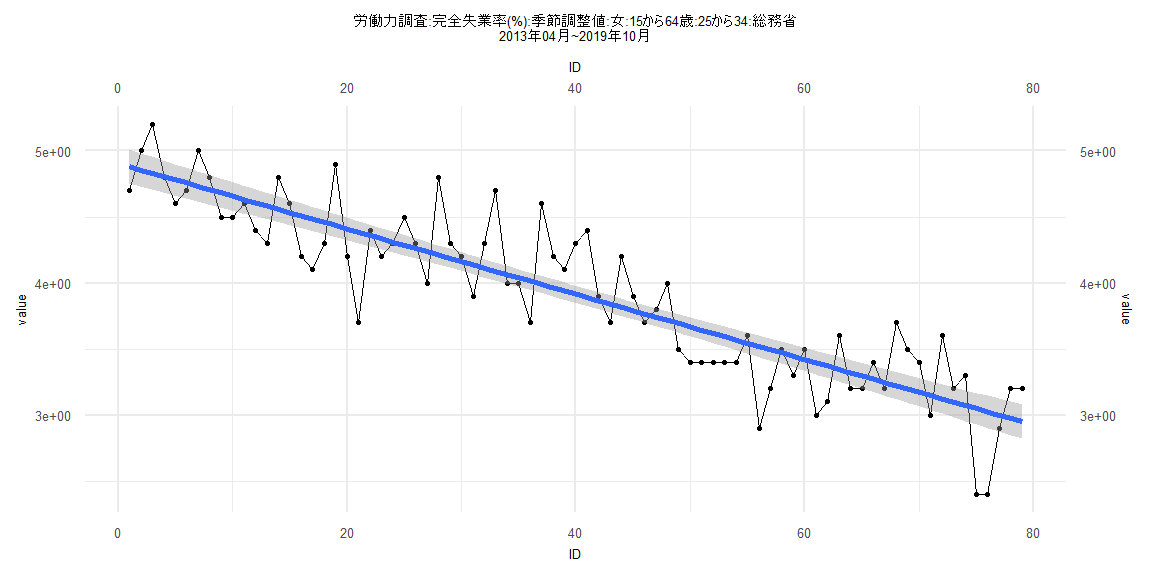
[1] "労働力調査:完全失業率(%):季節調整値:女:15から64歳:25から34:総務省"
     Jan Feb Mar Apr May Jun Jul Aug Sep Oct Nov Dec
1999                                             6.8
2000 7.2 6.9 6.6 6.8 6.1 6.2 6.4 6.5 6.5 6.6 6.2 6.0
2001 6.6 6.4 7.0 7.0 7.0 6.8 6.6 6.7 6.7 6.1 7.2 7.6
2002 7.1 7.4 7.7 6.9 7.2 7.8 7.8 7.3 7.3 7.4 7.0 7.4
2003 7.4 6.8 6.2 7.0 7.2 6.6 6.9 6.8 6.8 6.9 6.5 6.3
2004 5.5 6.1 5.7 6.2 6.1 6.4 5.8 5.8 5.7 5.9 5.2 5.1
2005 6.4 6.3 6.4 6.4 6.2 5.2 5.9 5.8 5.7 6.4 7.0 6.2
2006 5.1 4.9 5.6 4.8 5.0 5.4 5.4 5.6 5.6 4.9 5.0 5.4
2007 5.9 5.6 5.0 5.2 5.0 5.0 4.7 4.5 4.7 5.4 5.2 4.9
2008 4.8 5.4 5.5 5.5 5.3 5.5 5.5 5.7 5.5 4.8 5.0 5.6
2009 5.6 5.7 6.0 5.8 5.9 6.2 6.7 6.5 7.0 6.9 6.6 6.7
2010 6.5 6.0 5.7 5.9 5.7 5.4 5.3 5.8 5.6 5.9 6.1 5.6
2011 5.4 5.4 5.3 5.6 5.3 5.7 5.7 5.4 4.7 4.6 4.7 5.2
2012 5.7 5.3 5.7 5.1 5.2 4.6 4.3 4.8 5.4 4.8 4.9 5.1
2013 4.7 5.2 4.8 4.7 5.0 5.2 4.8 4.6 4.7 5.0 4.8 4.5
2014 4.5 4.6 4.4 4.3 4.8 4.6 4.2 4.1 4.3 4.9 4.2 3.7
2015 4.4 4.2 4.3 4.5 4.3 4.0 4.8 4.3 4.2 3.9 4.3 4.7
2016 4.0 4.0 3.7 4.6 4.2 4.1 4.3 4.4 3.9 3.7 4.2 3.9
2017 3.7 3.8 4.0 3.5 3.4 3.4 3.4 3.4 3.4 3.6 2.9 3.2
2018 3.5 3.3 3.5 3.0 3.1 3.6 3.2 3.2 3.4 3.2 3.7 3.5
2019 3.4 3.0 3.6 3.2 3.3 2.4 2.4 2.9 3.2 3.2
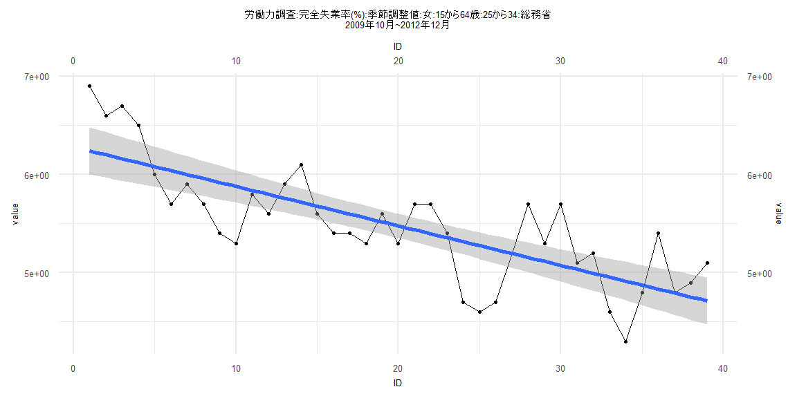
Call:
lm(formula = value ~ ID)

Residuals:
     Min       1Q   Median       3Q      Max
-0.67611 -0.24741  0.00421  0.28332  0.66000

Coefficients:
             Estimate Std. Error t value             Pr(>|t|)
(Intercept)  6.280162   0.123591  50.814 < 0.0000000000000002 ***
ID          -0.040162   0.005385  -7.458        0.00000000702 ***
---
Signif. codes:  0 '***' 0.001 '**' 0.01 '*' 0.05 '.' 0.1 ' ' 1

Residual standard error: 0.3785 on 37 degrees of freedom
Multiple R-squared:  0.6005,    Adjusted R-squared:  0.5897
F-statistic: 55.62 on 1 and 37 DF,  p-value: 0.000000007025


    Two-sample Kolmogorov-Smirnov test

data:  lm_residuals and rnorm(n = length(lm_residuals), mean = 0, sd = sd(lm_residuals))
D = 0.12821, p-value = 0.9114
alternative hypothesis: two-sided


    Durbin-Watson test

data:  value ~ ID
DW = 0.92372, p-value = 0.00005441
alternative hypothesis: true autocorrelation is greater than 0


    studentized Breusch-Pagan test

data:  value ~ ID
BP = 0.0092257, df = 1, p-value = 0.9235


    Box-Ljung test

data:  lm_residuals
X-squared = 9.8162, df = 1, p-value = 0.00173
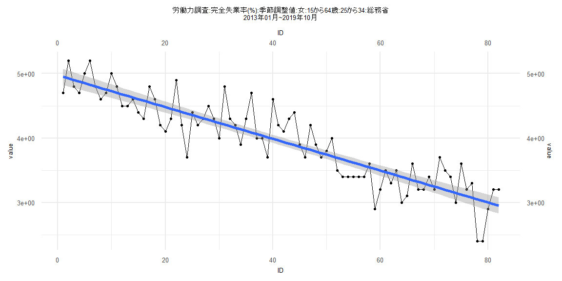
Call:
lm(formula = value ~ ID)

Residuals:
     Min       1Q   Median       3Q      Max
-0.68270 -0.18889 -0.01899  0.22100  0.61317

Coefficients:
             Estimate Std. Error t value            Pr(>|t|)
(Intercept)  4.974435   0.064106   77.60 <0.0000000000000002 ***
ID          -0.024656   0.001342  -18.38 <0.0000000000000002 ***
---
Signif. codes:  0 '***' 0.001 '**' 0.01 '*' 0.05 '.' 0.1 ' ' 1

Residual standard error: 0.2876 on 80 degrees of freedom
Multiple R-squared:  0.8084,    Adjusted R-squared:  0.8061
F-statistic: 337.6 on 1 and 80 DF,  p-value: < 0.00000000000000022


    Two-sample Kolmogorov-Smirnov test

data:  lm_residuals and rnorm(n = length(lm_residuals), mean = 0, sd = sd(lm_residuals))
D = 0.12195, p-value = 0.5785
alternative hypothesis: two-sided


    Durbin-Watson test

data:  value ~ ID
DW = 1.648, p-value = 0.04208
alternative hypothesis: true autocorrelation is greater than 0


    studentized Breusch-Pagan test

data:  value ~ ID
BP = 1.4619, df = 1, p-value = 0.2266


    Box-Ljung test

data:  lm_residuals
X-squared = 2.3619, df = 1, p-value = 0.1243
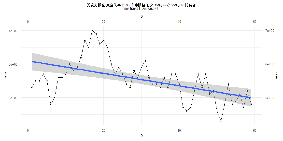
Call:
lm(formula = value ~ ID)

Residuals:
     Min       1Q   Median       3Q      Max
-1.18277 -0.32286  0.01842  0.30321  1.22219

Coefficients:
             Estimate Std. Error t value             Pr(>|t|)
(Intercept)  6.094565   0.135536  44.966 < 0.0000000000000002 ***
ID          -0.018632   0.003929  -4.742            0.0000146 ***
---
Signif. codes:  0 '***' 0.001 '**' 0.01 '*' 0.05 '.' 0.1 ' ' 1

Residual standard error: 0.5139 on 57 degrees of freedom
Multiple R-squared:  0.2829,    Adjusted R-squared:  0.2703
F-statistic: 22.49 on 1 and 57 DF,  p-value: 0.00001455


    Two-sample Kolmogorov-Smirnov test

data:  lm_residuals and rnorm(n = length(lm_residuals), mean = 0, sd = sd(lm_residuals))
D = 0.10169, p-value = 0.9239
alternative hypothesis: two-sided


    Durbin-Watson test

data:  value ~ ID
DW = 0.4883, p-value = 0.0000000000001814
alternative hypothesis: true autocorrelation is greater than 0


    studentized Breusch-Pagan test

data:  value ~ ID
BP = 7.143, df = 1, p-value = 0.007526


    Box-Ljung test

data:  lm_residuals
X-squared = 33.484, df = 1, p-value = 0.000000007184
Call:
lm(formula = value ~ ID)

Residuals:
     Min       1Q   Median       3Q      Max
-0.68515 -0.18727 -0.01094  0.21926  0.61167

Coefficients:
            Estimate Std. Error t value            Pr(>|t|)
(Intercept)  4.90458    0.06585   74.49 <0.0000000000000002 ***
ID          -0.02474    0.00143  -17.30 <0.0000000000000002 ***
---
Signif. codes:  0 '***' 0.001 '**' 0.01 '*' 0.05 '.' 0.1 ' ' 1

Residual standard error: 0.2898 on 77 degrees of freedom
Multiple R-squared:  0.7953,    Adjusted R-squared:  0.7926
F-statistic: 299.2 on 1 and 77 DF,  p-value: < 0.00000000000000022


    Two-sample Kolmogorov-Smirnov test

data:  lm_residuals and rnorm(n = length(lm_residuals), mean = 0, sd = sd(lm_residuals))
D = 0.075949, p-value = 0.978
alternative hypothesis: two-sided


    Durbin-Watson test

data:  value ~ ID
DW = 1.6206, p-value = 0.03397
alternative hypothesis: true autocorrelation is greater than 0


    studentized Breusch-Pagan test

data:  value ~ ID
BP = 1.1918, df = 1, p-value = 0.275


    Box-Ljung test

data:  lm_residuals
X-squared = 2.729, df = 1, p-value = 0.09854