Analysis
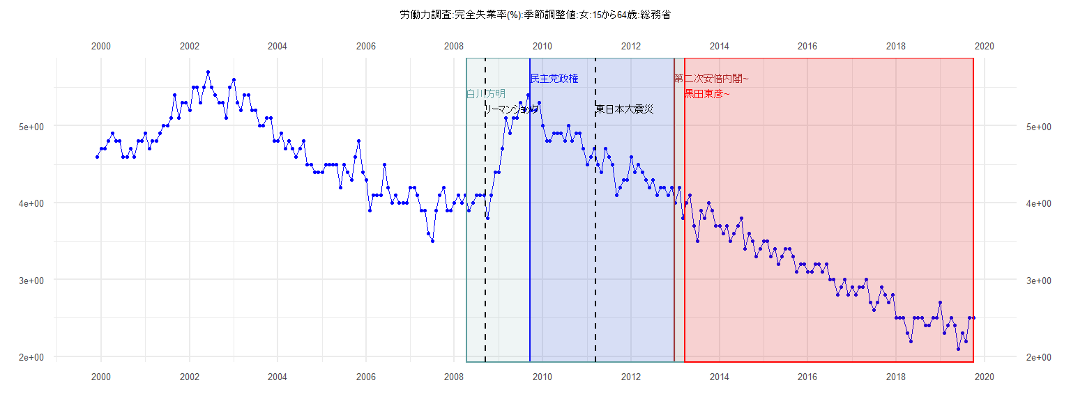
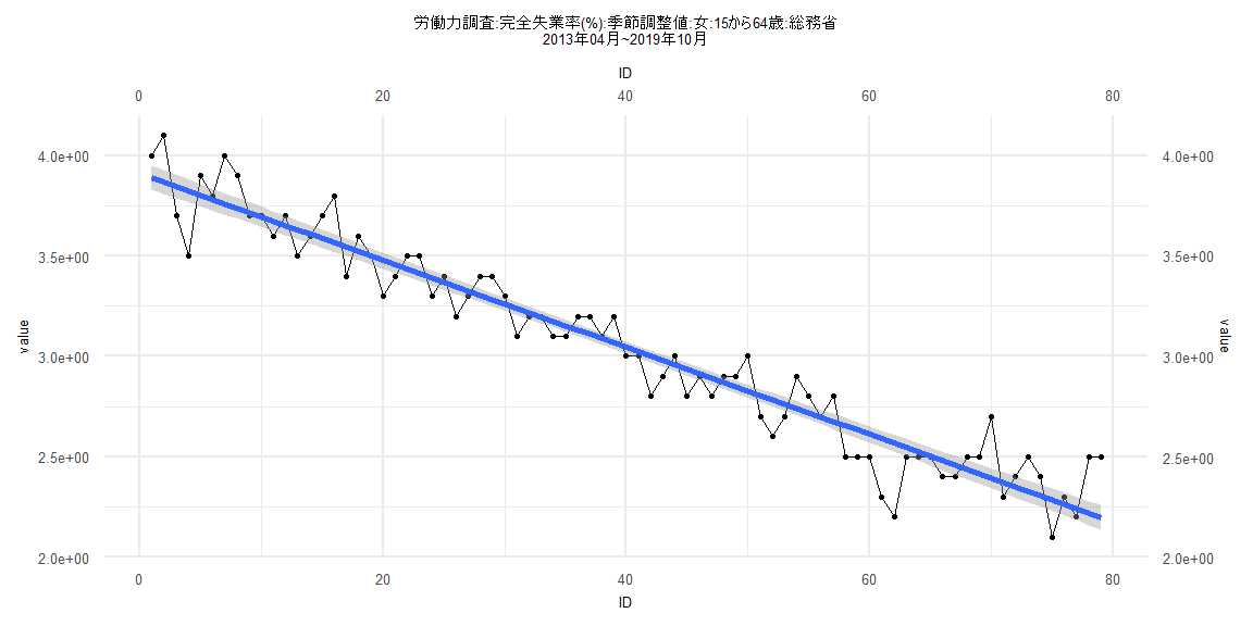
[1] "労働力調査:完全失業率(%):季節調整値:女:15から64歳:総務省"
     Jan Feb Mar Apr May Jun Jul Aug Sep Oct Nov Dec
1999                                             4.6
2000 4.7 4.7 4.8 4.9 4.8 4.8 4.6 4.6 4.7 4.6 4.8 4.8
2001 4.9 4.7 4.8 4.8 4.9 5.0 5.0 5.1 5.4 5.1 5.3 5.3
2002 5.2 5.5 5.5 5.3 5.5 5.7 5.5 5.4 5.3 5.3 5.1 5.5
2003 5.6 5.3 5.2 5.4 5.4 5.2 5.2 5.0 5.0 5.1 5.1 4.8
2004 4.8 4.9 4.7 4.8 4.7 4.6 4.7 4.8 4.5 4.5 4.4 4.4
2005 4.4 4.5 4.5 4.5 4.5 4.2 4.5 4.4 4.3 4.6 4.8 4.4
2006 4.3 3.9 4.1 4.1 4.1 4.5 4.2 4.0 4.1 4.0 4.0 4.0
2007 4.2 4.2 4.1 3.9 3.9 3.6 3.5 3.9 4.1 4.2 3.9 3.9
2008 4.0 4.1 4.0 4.1 3.9 4.0 4.1 4.1 4.1 3.8 4.1 4.4
2009 4.4 4.7 5.1 4.9 5.1 5.1 5.3 5.2 5.4 5.2 5.2 5.3
2010 5.0 4.8 4.8 4.9 4.9 4.9 4.8 5.0 4.8 4.9 4.9 4.7
2011 4.5 4.6 4.7 4.5 4.4 4.7 4.6 4.5 4.1 4.2 4.3 4.3
2012 4.6 4.4 4.5 4.4 4.3 4.2 4.3 4.1 4.2 4.2 4.1 4.2
2013 4.0 4.2 3.8 4.0 4.1 3.7 3.5 3.9 3.8 4.0 3.9 3.7
2014 3.7 3.6 3.7 3.5 3.6 3.7 3.8 3.4 3.6 3.5 3.3 3.4
2015 3.5 3.5 3.3 3.4 3.2 3.3 3.4 3.4 3.3 3.1 3.2 3.2
2016 3.1 3.1 3.2 3.2 3.1 3.2 3.0 3.0 2.8 2.9 3.0 2.8
2017 2.9 2.8 2.9 2.9 3.0 2.7 2.6 2.7 2.9 2.8 2.7 2.8
2018 2.5 2.5 2.5 2.3 2.2 2.5 2.5 2.5 2.4 2.4 2.5 2.5
2019 2.7 2.3 2.4 2.5 2.4 2.1 2.3 2.2 2.5 2.5
Call:
lm(formula = value ~ ID)

Residuals:
     Min       1Q   Median       3Q      Max
-0.38302 -0.07966 -0.00318  0.10354  0.25669

Coefficients:
             Estimate Std. Error t value             Pr(>|t|)
(Intercept)  5.123347   0.045531  112.53 < 0.0000000000000002 ***
ID          -0.026680   0.001984  -13.45 0.000000000000000811 ***
---
Signif. codes:  0 '***' 0.001 '**' 0.01 '*' 0.05 '.' 0.1 ' ' 1

Residual standard error: 0.1394 on 37 degrees of freedom
Multiple R-squared:  0.8302,    Adjusted R-squared:  0.8256
F-statistic: 180.8 on 1 and 37 DF,  p-value: 0.0000000000000008112


    Two-sample Kolmogorov-Smirnov test

data:  lm_residuals and rnorm(n = length(lm_residuals), mean = 0, sd = sd(lm_residuals))
D = 0.28205, p-value = 0.08974
alternative hypothesis: two-sided


    Durbin-Watson test

data:  value ~ ID
DW = 1.27, p-value = 0.00523
alternative hypothesis: true autocorrelation is greater than 0


    studentized Breusch-Pagan test

data:  value ~ ID
BP = 0.14068, df = 1, p-value = 0.7076


    Box-Ljung test

data:  lm_residuals
X-squared = 5.0973, df = 1, p-value = 0.02396
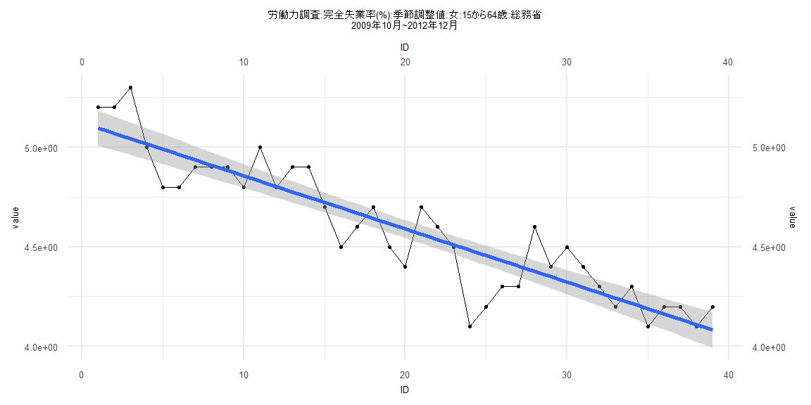
Call:
lm(formula = value ~ ID)

Residuals:
     Min       1Q   Median       3Q      Max
-0.36602 -0.08071 -0.00111  0.08570  0.30870

Coefficients:
              Estimate Std. Error t value            Pr(>|t|)
(Intercept)  3.9856369  0.0305357  130.52 <0.0000000000000002 ***
ID          -0.0218402  0.0006392  -34.17 <0.0000000000000002 ***
---
Signif. codes:  0 '***' 0.001 '**' 0.01 '*' 0.05 '.' 0.1 ' ' 1

Residual standard error: 0.137 on 80 degrees of freedom
Multiple R-squared:  0.9359,    Adjusted R-squared:  0.9351
F-statistic:  1168 on 1 and 80 DF,  p-value: < 0.00000000000000022


    Two-sample Kolmogorov-Smirnov test

data:  lm_residuals and rnorm(n = length(lm_residuals), mean = 0, sd = sd(lm_residuals))
D = 0.085366, p-value = 0.9286
alternative hypothesis: two-sided


    Durbin-Watson test

data:  value ~ ID
DW = 1.5473, p-value = 0.01392
alternative hypothesis: true autocorrelation is greater than 0


    studentized Breusch-Pagan test

data:  value ~ ID
BP = 0.61433, df = 1, p-value = 0.4332


    Box-Ljung test

data:  lm_residuals
X-squared = 3.2293, df = 1, p-value = 0.07233
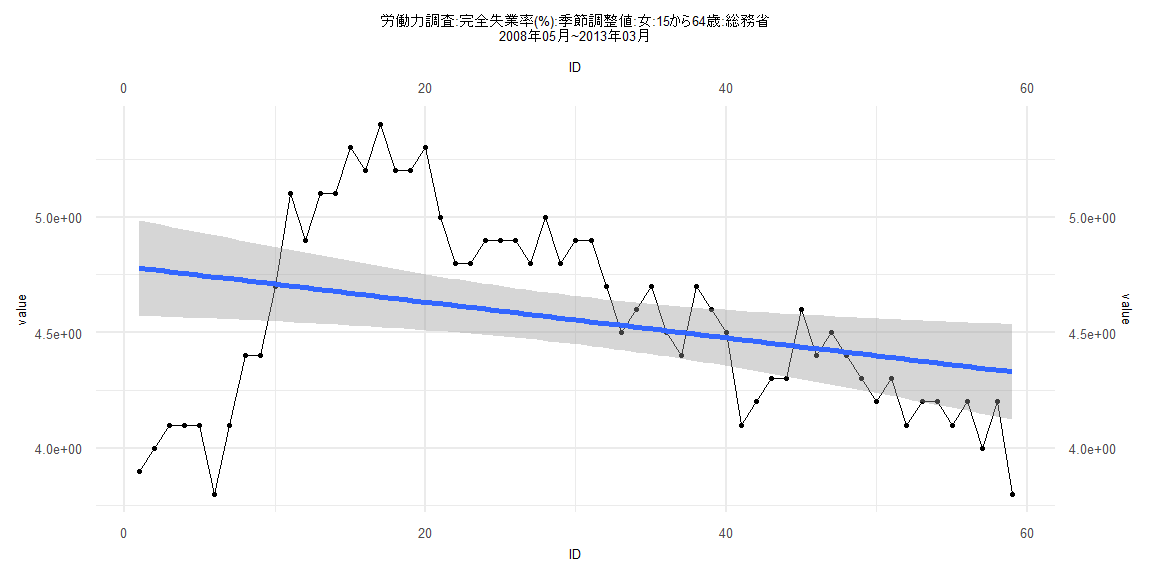
Call:
lm(formula = value ~ ID)

Residuals:
     Min       1Q   Median       3Q      Max
-0.94009 -0.23000 -0.00777  0.30317  0.74509

Coefficients:
             Estimate Std. Error t value            Pr(>|t|)
(Intercept)  4.786558   0.105722  45.275 <0.0000000000000002 ***
ID          -0.007744   0.003065  -2.527              0.0143 *
---
Signif. codes:  0 '***' 0.001 '**' 0.01 '*' 0.05 '.' 0.1 ' ' 1

Residual standard error: 0.4009 on 57 degrees of freedom
Multiple R-squared:  0.1007,    Adjusted R-squared:  0.08495
F-statistic: 6.385 on 1 and 57 DF,  p-value: 0.01431


    Two-sample Kolmogorov-Smirnov test

data:  lm_residuals and rnorm(n = length(lm_residuals), mean = 0, sd = sd(lm_residuals))
D = 0.084746, p-value = 0.9854
alternative hypothesis: two-sided


    Durbin-Watson test

data:  value ~ ID
DW = 0.2109, p-value < 0.00000000000000022
alternative hypothesis: true autocorrelation is greater than 0


    studentized Breusch-Pagan test

data:  value ~ ID
BP = 23.749, df = 1, p-value = 0.000001097


    Box-Ljung test

data:  lm_residuals
X-squared = 43.48, df = 1, p-value = 0.00000000004283
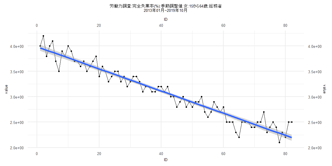
Call:
lm(formula = value ~ ID)

Residuals:
     Min       1Q   Median       3Q      Max
-0.36773 -0.08020  0.00078  0.08567  0.30557

Coefficients:
              Estimate Std. Error t value            Pr(>|t|)
(Intercept)  3.9108082  0.0308213  126.89 <0.0000000000000002 ***
ID          -0.0216626  0.0006694  -32.36 <0.0000000000000002 ***
---
Signif. codes:  0 '***' 0.001 '**' 0.01 '*' 0.05 '.' 0.1 ' ' 1

Residual standard error: 0.1357 on 77 degrees of freedom
Multiple R-squared:  0.9315,    Adjusted R-squared:  0.9306
F-statistic:  1047 on 1 and 77 DF,  p-value: < 0.00000000000000022


    Two-sample Kolmogorov-Smirnov test

data:  lm_residuals and rnorm(n = length(lm_residuals), mean = 0, sd = sd(lm_residuals))
D = 0.13924, p-value = 0.4302
alternative hypothesis: two-sided


    Durbin-Watson test

data:  value ~ ID
DW = 1.4686, p-value = 0.005673
alternative hypothesis: true autocorrelation is greater than 0


    studentized Breusch-Pagan test

data:  value ~ ID
BP = 0.94764, df = 1, p-value = 0.3303


    Box-Ljung test

data:  lm_residuals
X-squared = 4.3204, df = 1, p-value = 0.03766