Analysis
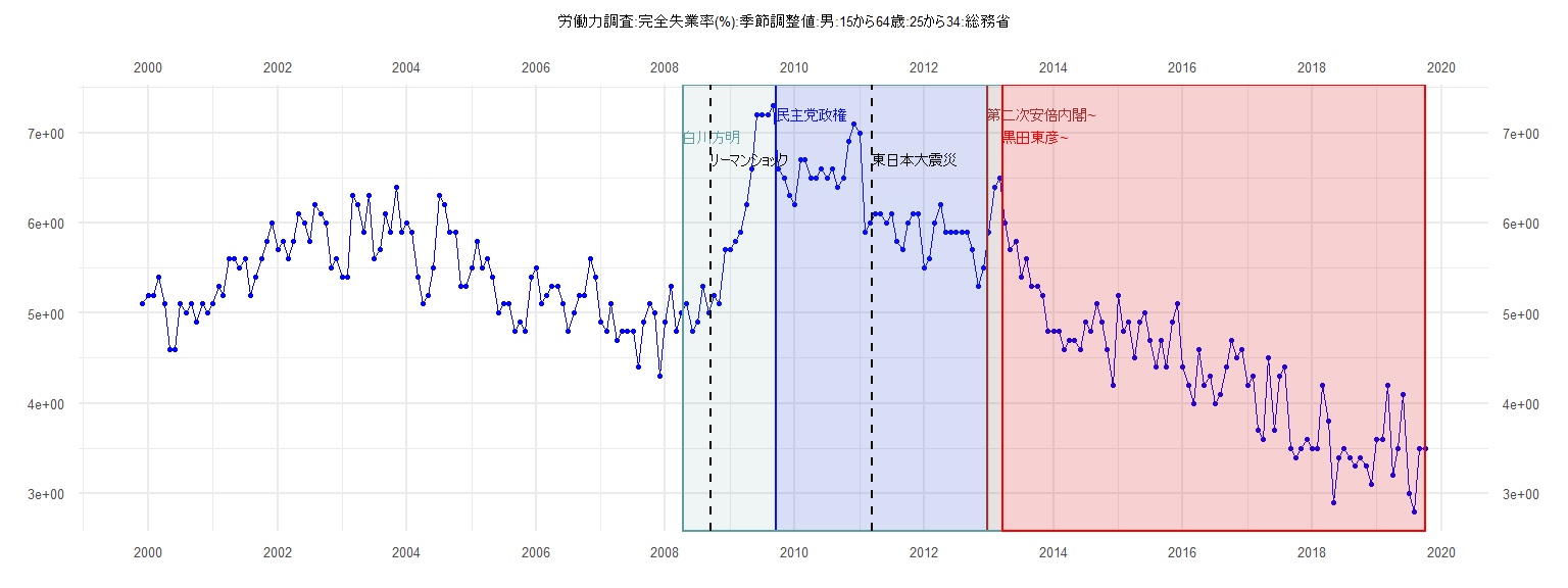
[1] "労働力調査:完全失業率(%):季節調整値:男:15から64歳:25から34:総務省"
     Jan Feb Mar Apr May Jun Jul Aug Sep Oct Nov Dec
1999                                             5.1
2000 5.2 5.2 5.4 5.1 4.6 4.6 5.1 5.0 5.1 4.9 5.1 5.0
2001 5.1 5.3 5.2 5.6 5.6 5.5 5.6 5.2 5.4 5.6 5.8 6.0
2002 5.7 5.8 5.6 5.8 6.1 6.0 5.8 6.2 6.1 6.0 5.5 5.6
2003 5.4 5.4 6.3 6.2 5.9 6.3 5.6 5.7 6.1 5.9 6.4 5.9
2004 6.0 5.9 5.4 5.1 5.2 5.5 6.3 6.2 5.9 5.9 5.3 5.3
2005 5.5 5.8 5.5 5.6 5.4 5.0 5.1 5.1 4.8 4.9 4.8 5.4
2006 5.5 5.1 5.2 5.3 5.3 5.1 4.8 5.0 5.2 5.2 5.6 5.4
2007 4.9 4.8 5.1 4.7 4.8 4.8 4.8 4.4 4.9 5.1 5.0 4.3
2008 4.9 5.3 4.8 5.0 5.1 4.8 4.9 5.3 5.0 5.2 5.1 5.7
2009 5.7 5.8 5.9 6.2 6.6 7.2 7.2 7.2 7.3 6.6 6.5 6.3
2010 6.2 6.7 6.7 6.5 6.5 6.6 6.5 6.6 6.4 6.5 6.9 7.1
2011 7.0 5.9 6.0 6.1 6.1 6.0 6.1 5.8 5.7 6.0 6.1 6.1
2012 5.5 5.6 6.0 6.2 5.9 5.9 5.9 5.9 5.9 5.7 5.3 5.5
2013 5.9 6.4 6.5 6.0 5.7 5.8 5.4 5.6 5.3 5.3 5.2 4.8
2014 4.8 4.8 4.6 4.7 4.7 4.6 4.9 4.8 5.1 4.9 4.6 4.2
2015 5.2 4.8 4.9 4.5 4.9 5.0 4.7 4.4 4.7 4.4 4.9 5.1
2016 4.4 4.2 4.0 4.6 4.2 4.3 4.0 4.1 4.4 4.7 4.5 4.6
2017 4.2 4.3 3.7 3.6 4.5 3.7 4.3 4.4 3.5 3.4 3.5 3.6
2018 3.5 3.5 4.2 3.8 2.9 3.4 3.5 3.4 3.3 3.4 3.3 3.1
2019 3.6 3.6 4.2 3.2 3.5 4.1 3.0 2.8 3.5 3.5
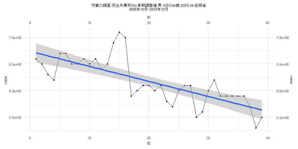
Call:
lm(formula = value ~ ID)

Residuals:
     Min       1Q   Median       3Q      Max
-0.44796 -0.16491 -0.00076  0.12279  0.78414

Coefficients:
            Estimate Std. Error t value             Pr(>|t|)
(Intercept)  6.74035    0.09294  72.520 < 0.0000000000000002 ***
ID          -0.02830    0.00405  -6.988         0.0000000295 ***
---
Signif. codes:  0 '***' 0.001 '**' 0.01 '*' 0.05 '.' 0.1 ' ' 1

Residual standard error: 0.2847 on 37 degrees of freedom
Multiple R-squared:  0.5689,    Adjusted R-squared:  0.5572
F-statistic: 48.83 on 1 and 37 DF,  p-value: 0.00000002945


    Two-sample Kolmogorov-Smirnov test

data:  lm_residuals and rnorm(n = length(lm_residuals), mean = 0, sd = sd(lm_residuals))
D = 0.12821, p-value = 0.9114
alternative hypothesis: two-sided


    Durbin-Watson test

data:  value ~ ID
DW = 0.98669, p-value = 0.0001499
alternative hypothesis: true autocorrelation is greater than 0


    studentized Breusch-Pagan test

data:  value ~ ID
BP = 0.35084, df = 1, p-value = 0.5536


    Box-Ljung test

data:  lm_residuals
X-squared = 10.581, df = 1, p-value = 0.001143
Call:
lm(formula = value ~ ID)

Residuals:
     Min       1Q   Median       3Q      Max
-0.73978 -0.26463 -0.06359  0.23435  0.97358

Coefficients:
             Estimate Std. Error t value            Pr(>|t|)
(Intercept)  5.617706   0.082818   67.83 <0.0000000000000002 ***
ID          -0.030430   0.001733  -17.55 <0.0000000000000002 ***
---
Signif. codes:  0 '***' 0.001 '**' 0.01 '*' 0.05 '.' 0.1 ' ' 1

Residual standard error: 0.3716 on 80 degrees of freedom
Multiple R-squared:  0.7939,    Adjusted R-squared:  0.7913
F-statistic: 308.1 on 1 and 80 DF,  p-value: < 0.00000000000000022


    Two-sample Kolmogorov-Smirnov test

data:  lm_residuals and rnorm(n = length(lm_residuals), mean = 0, sd = sd(lm_residuals))
D = 0.097561, p-value = 0.8332
alternative hypothesis: two-sided


    Durbin-Watson test

data:  value ~ ID
DW = 1.2612, p-value = 0.0001604
alternative hypothesis: true autocorrelation is greater than 0


    studentized Breusch-Pagan test

data:  value ~ ID
BP = 0.20902, df = 1, p-value = 0.6475


    Box-Ljung test

data:  lm_residuals
X-squared = 10.93, df = 1, p-value = 0.0009463
Call:
lm(formula = value ~ ID)

Residuals:
     Min       1Q   Median       3Q      Max
-1.23710 -0.33519 -0.02891  0.41372  1.23011

Coefficients:
            Estimate Std. Error t value            Pr(>|t|)
(Intercept) 6.032729   0.159876  37.734 <0.0000000000000002 ***
ID          0.002186   0.004635   0.472               0.639
---
Signif. codes:  0 '***' 0.001 '**' 0.01 '*' 0.05 '.' 0.1 ' ' 1

Residual standard error: 0.6062 on 57 degrees of freedom
Multiple R-squared:  0.003887,  Adjusted R-squared:  -0.01359
F-statistic: 0.2224 on 1 and 57 DF,  p-value: 0.639


    Two-sample Kolmogorov-Smirnov test

data:  lm_residuals and rnorm(n = length(lm_residuals), mean = 0, sd = sd(lm_residuals))
D = 0.13559, p-value = 0.6544
alternative hypothesis: two-sided


    Durbin-Watson test

data:  value ~ ID
DW = 0.25273, p-value < 0.00000000000000022
alternative hypothesis: true autocorrelation is greater than 0


    studentized Breusch-Pagan test

data:  value ~ ID
BP = 14.962, df = 1, p-value = 0.0001097


    Box-Ljung test

data:  lm_residuals
X-squared = 44.837, df = 1, p-value = 0.00000000002142
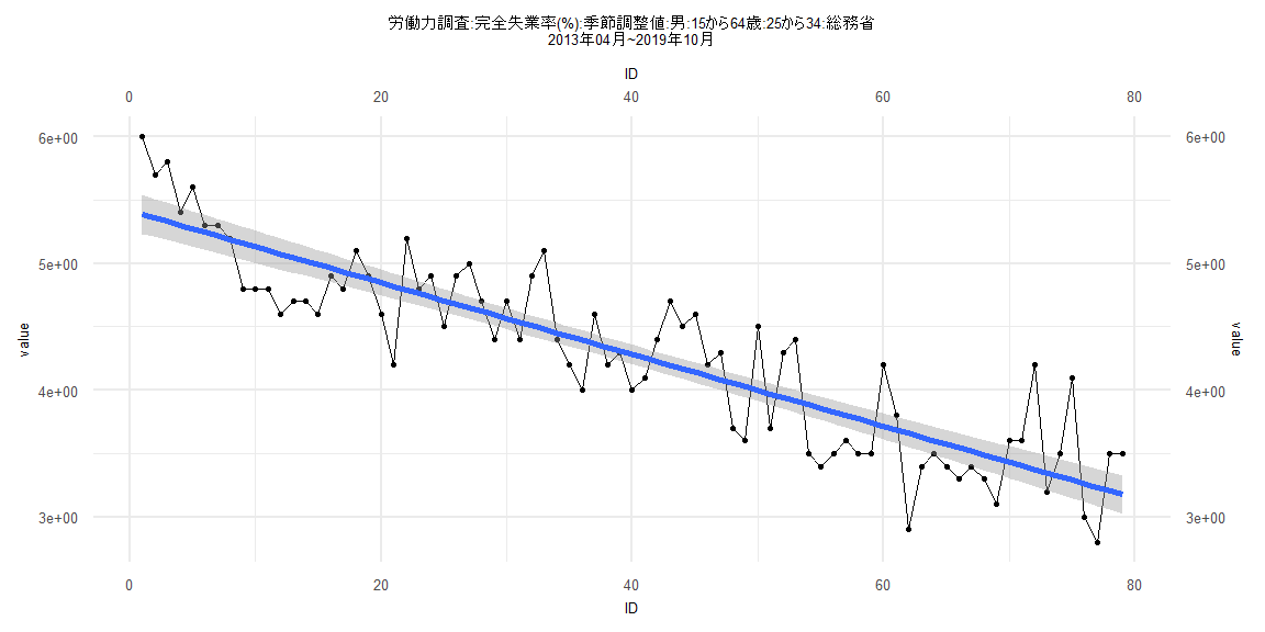
Call:
lm(formula = value ~ ID)

Residuals:
    Min      1Q  Median      3Q     Max
-0.7592 -0.2667 -0.0522  0.2270  0.8240

Coefficients:
             Estimate Std. Error t value            Pr(>|t|)
(Intercept)  5.415093   0.077869   69.54 <0.0000000000000002 ***
ID          -0.028320   0.001691  -16.75 <0.0000000000000002 ***
---
Signif. codes:  0 '***' 0.001 '**' 0.01 '*' 0.05 '.' 0.1 ' ' 1

Residual standard error: 0.3428 on 77 degrees of freedom
Multiple R-squared:  0.7846,    Adjusted R-squared:  0.7818
F-statistic: 280.4 on 1 and 77 DF,  p-value: < 0.00000000000000022


    Two-sample Kolmogorov-Smirnov test

data:  lm_residuals and rnorm(n = length(lm_residuals), mean = 0, sd = sd(lm_residuals))
D = 0.11392, p-value = 0.6878
alternative hypothesis: two-sided


    Durbin-Watson test

data:  value ~ ID
DW = 1.4823, p-value = 0.006804
alternative hypothesis: true autocorrelation is greater than 0


    studentized Breusch-Pagan test

data:  value ~ ID
BP = 1.6203, df = 1, p-value = 0.2031


    Box-Ljung test

data:  lm_residuals
X-squared = 4.4279, df = 1, p-value = 0.03536