Analysis
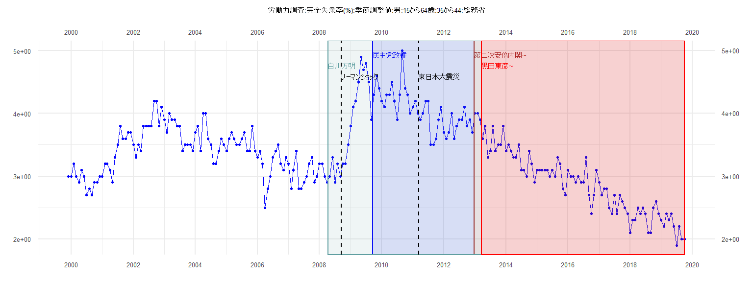
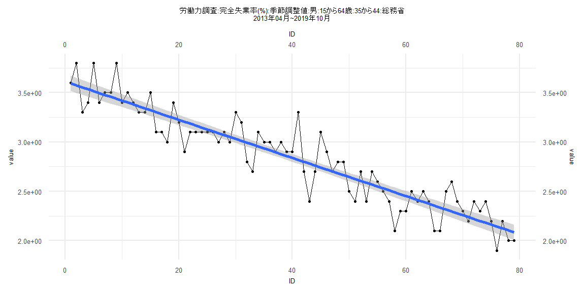
[1] "労働力調査:完全失業率(%):季節調整値:男:15から64歳:35から44:総務省"
     Jan Feb Mar Apr May Jun Jul Aug Sep Oct Nov Dec
1999                                             3.0
2000 3.0 3.2 3.0 2.9 3.1 3.0 2.7 2.8 2.7 2.9 2.9 3.0
2001 3.0 3.2 3.2 3.1 2.9 3.3 3.5 3.8 3.6 3.6 3.7 3.7
2002 3.5 3.3 3.5 3.4 3.8 3.8 3.8 3.8 4.2 4.2 3.8 4.1
2003 3.9 3.7 4.0 3.9 3.9 3.8 3.8 3.4 3.5 3.5 3.5 3.4
2004 3.7 3.8 3.4 4.0 4.0 3.6 3.5 3.2 3.2 3.4 3.6 3.5
2005 3.4 3.6 3.7 3.6 3.5 3.5 3.6 3.7 3.4 3.4 3.8 3.4
2006 3.3 3.4 3.2 2.5 2.8 3.0 3.3 3.4 3.5 3.2 3.1 3.3
2007 3.2 2.8 3.1 3.4 2.8 2.8 2.9 3.0 3.2 3.3 2.9 3.0
2008 3.2 3.2 3.0 2.9 3.0 3.3 2.9 3.2 3.0 3.2 3.2 3.5
2009 3.8 4.1 4.2 4.5 4.9 4.7 4.8 4.5 3.9 4.3 4.6 4.4
2010 4.2 4.1 4.3 4.3 4.5 4.2 3.9 4.3 5.0 4.4 4.3 4.0
2011 4.1 4.2 4.0 3.9 4.0 4.2 4.2 3.5 3.5 3.6 3.9 4.1
2012 3.7 3.6 3.7 4.0 3.6 3.8 3.9 3.9 4.1 3.8 3.9 3.7
2013 4.0 4.0 3.9 3.6 3.8 3.3 3.4 3.8 3.4 3.5 3.5 3.8
2014 3.4 3.5 3.4 3.3 3.3 3.5 3.1 3.1 3.0 3.4 3.2 2.9
2015 3.1 3.1 3.1 3.1 3.1 3.0 3.1 3.0 3.3 3.2 2.8 2.7
2016 3.1 3.0 3.0 2.9 3.0 2.9 2.9 3.3 2.7 2.4 2.7 3.1
2017 2.9 2.7 2.8 2.8 2.5 2.4 2.7 2.4 2.7 2.6 2.5 2.4
2018 2.1 2.3 2.3 2.5 2.4 2.5 2.4 2.1 2.1 2.5 2.6 2.4
2019 2.3 2.2 2.4 2.3 2.4 2.2 1.9 2.2 2.0 2.0
Call:
lm(formula = value ~ ID)

Residuals:
     Min       1Q   Median       3Q      Max
-0.48717 -0.15001  0.00088  0.15342  0.80596

Coefficients:
             Estimate Std. Error t value             Pr(>|t|)
(Intercept)  4.419703   0.079417  55.652 < 0.0000000000000002 ***
ID          -0.018806   0.003461  -5.434           0.00000366 ***
---
Signif. codes:  0 '***' 0.001 '**' 0.01 '*' 0.05 '.' 0.1 ' ' 1

Residual standard error: 0.2432 on 37 degrees of freedom
Multiple R-squared:  0.4439,    Adjusted R-squared:  0.4288
F-statistic: 29.53 on 1 and 37 DF,  p-value: 0.000003664


    Two-sample Kolmogorov-Smirnov test

data:  lm_residuals and rnorm(n = length(lm_residuals), mean = 0, sd = sd(lm_residuals))
D = 0.23077, p-value = 0.2523
alternative hypothesis: two-sided


    Durbin-Watson test

data:  value ~ ID
DW = 1.3481, p-value = 0.01106
alternative hypothesis: true autocorrelation is greater than 0


    studentized Breusch-Pagan test

data:  value ~ ID
BP = 0.059233, df = 1, p-value = 0.8077


    Box-Ljung test

data:  lm_residuals
X-squared = 4.4054, df = 1, p-value = 0.03583
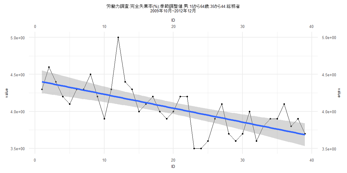
Call:
lm(formula = value ~ ID)

Residuals:
    Min      1Q  Median      3Q     Max
-0.3896 -0.1120 -0.0098  0.1233  0.4700

Coefficients:
              Estimate Std. Error t value            Pr(>|t|)
(Intercept)  3.7186089  0.0405775   91.64 <0.0000000000000002 ***
ID          -0.0201957  0.0008493  -23.78 <0.0000000000000002 ***
---
Signif. codes:  0 '***' 0.001 '**' 0.01 '*' 0.05 '.' 0.1 ' ' 1

Residual standard error: 0.182 on 80 degrees of freedom
Multiple R-squared:  0.876, Adjusted R-squared:  0.8745
F-statistic: 565.4 on 1 and 80 DF,  p-value: < 0.00000000000000022


    Two-sample Kolmogorov-Smirnov test

data:  lm_residuals and rnorm(n = length(lm_residuals), mean = 0, sd = sd(lm_residuals))
D = 0.14634, p-value = 0.3453
alternative hypothesis: two-sided


    Durbin-Watson test

data:  value ~ ID
DW = 1.5813, p-value = 0.02071
alternative hypothesis: true autocorrelation is greater than 0


    studentized Breusch-Pagan test

data:  value ~ ID
BP = 0.7056, df = 1, p-value = 0.4009


    Box-Ljung test

data:  lm_residuals
X-squared = 3.1179, df = 1, p-value = 0.07744
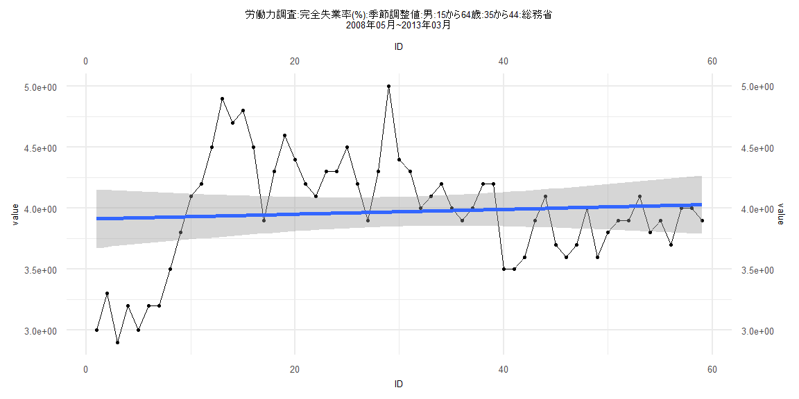
Call:
lm(formula = value ~ ID)

Residuals:
     Min       1Q   Median       3Q      Max
-1.01753 -0.30298 -0.00695  0.29670  1.03080

Coefficients:
            Estimate Std. Error t value            Pr(>|t|)
(Intercept) 3.911572   0.122575  31.912 <0.0000000000000002 ***
ID          0.001987   0.003553   0.559               0.578
---
Signif. codes:  0 '***' 0.001 '**' 0.01 '*' 0.05 '.' 0.1 ' ' 1

Residual standard error: 0.4648 on 57 degrees of freedom
Multiple R-squared:  0.005457,  Adjusted R-squared:  -0.01199
F-statistic: 0.3128 on 1 and 57 DF,  p-value: 0.5782


    Two-sample Kolmogorov-Smirnov test

data:  lm_residuals and rnorm(n = length(lm_residuals), mean = 0, sd = sd(lm_residuals))
D = 0.11864, p-value = 0.8052
alternative hypothesis: two-sided


    Durbin-Watson test

data:  value ~ ID
DW = 0.37899, p-value < 0.00000000000000022
alternative hypothesis: true autocorrelation is greater than 0


    studentized Breusch-Pagan test

data:  value ~ ID
BP = 20.144, df = 1, p-value = 0.000007181


    Box-Ljung test

data:  lm_residuals
X-squared = 37.361, df = 1, p-value = 0.0000000009819
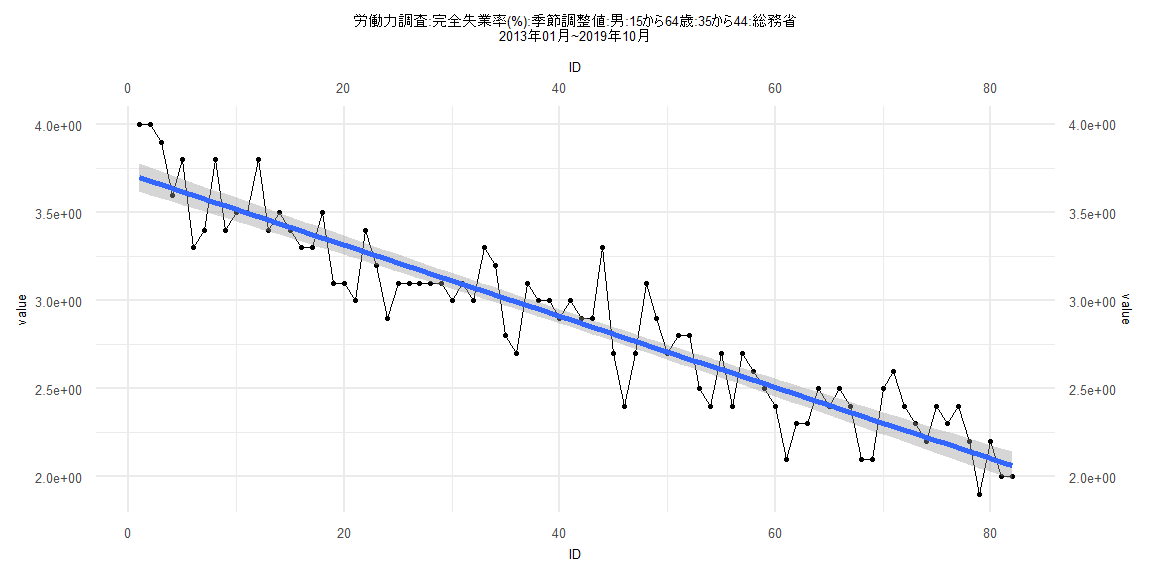
Call:
lm(formula = value ~ ID)

Residuals:
     Min       1Q   Median       3Q      Max
-0.39129 -0.10263  0.00277  0.11038  0.48009

Coefficients:
              Estimate Std. Error t value            Pr(>|t|)
(Intercept)  3.6124635  0.0397534   90.87 <0.0000000000000002 ***
ID          -0.0193306  0.0008634  -22.39 <0.0000000000000002 ***
---
Signif. codes:  0 '***' 0.001 '**' 0.01 '*' 0.05 '.' 0.1 ' ' 1

Residual standard error: 0.175 on 77 degrees of freedom
Multiple R-squared:  0.8668,    Adjusted R-squared:  0.8651
F-statistic: 501.3 on 1 and 77 DF,  p-value: < 0.00000000000000022


    Two-sample Kolmogorov-Smirnov test

data:  lm_residuals and rnorm(n = length(lm_residuals), mean = 0, sd = sd(lm_residuals))
D = 0.12658, p-value = 0.5543
alternative hypothesis: two-sided


    Durbin-Watson test

data:  value ~ ID
DW = 1.7419, p-value = 0.1015
alternative hypothesis: true autocorrelation is greater than 0


    studentized Breusch-Pagan test

data:  value ~ ID
BP = 0.0062363, df = 1, p-value = 0.9371


    Box-Ljung test

data:  lm_residuals
X-squared = 1.3336, df = 1, p-value = 0.2482