Analysis
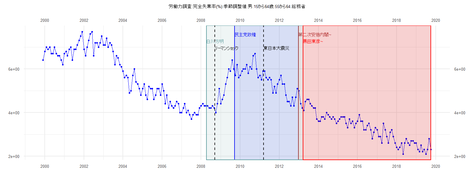
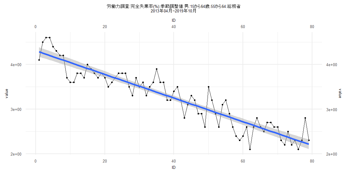
[1] "労働力調査:完全失業率(%):季節調整値:男:15から64歳:55から64:総務省"
     Jan Feb Mar Apr May Jun Jul Aug Sep Oct Nov Dec
1999                                             6.4
2000 6.8 7.0 6.9 7.0 6.7 6.7 7.0 6.7 6.6 6.6 6.4 6.2
2001 6.7 6.8 6.6 6.9 7.0 6.4 6.9 6.9 7.1 7.3 7.5 7.7
2002 6.9 6.6 7.0 7.3 7.6 7.7 6.6 7.2 7.2 7.0 7.2 7.5
2003 7.1 7.1 7.4 7.0 7.2 7.1 6.8 6.2 6.6 6.5 6.2 6.1
2004 5.9 5.6 5.7 5.6 4.9 5.0 5.7 6.0 5.4 5.3 5.1 4.8
2005 5.1 5.3 4.8 4.6 5.2 5.1 5.1 4.6 4.8 5.1 5.1 4.8
2006 5.3 5.0 4.4 4.8 4.2 4.5 4.3 4.2 4.3 4.5 4.4 4.0
2007 4.0 4.2 4.4 4.0 4.1 3.9 3.7 3.9 4.0 3.9 3.9 4.2
2008 4.3 4.4 4.3 4.3 4.3 4.2 4.2 4.3 4.2 4.0 4.4 5.1
2009 4.4 4.6 4.8 5.3 5.6 6.0 5.9 6.4 6.0 5.7 6.2 5.6
2010 5.7 5.9 6.0 6.0 6.2 5.8 6.1 6.0 6.6 6.7 6.0 5.6
2011 5.7 5.5 5.9 5.9 5.6 5.5 5.6 5.5 4.9 5.2 4.9 5.3
2012 5.5 5.7 5.3 5.3 4.8 4.5 4.5 4.3 4.7 4.3 4.7 5.1
2013 5.0 4.4 4.2 4.1 4.5 4.6 4.6 4.4 4.3 4.2 4.2 3.7
2014 3.6 3.6 3.8 3.8 3.7 4.0 3.9 3.8 3.7 3.8 3.7 3.5
2015 3.6 3.7 3.8 3.8 3.8 3.5 3.3 3.7 3.5 3.6 3.3 3.5
2016 3.6 3.9 3.6 3.6 3.2 3.2 3.4 3.5 3.2 2.8 3.1 3.3
2017 3.2 2.9 2.9 2.6 3.5 3.2 2.9 2.6 3.1 3.2 2.9 2.6
2018 2.4 2.3 2.4 2.6 2.1 2.6 2.8 2.6 2.5 2.7 2.7 2.6
2019 2.6 2.3 2.2 2.5 2.2 2.3 2.1 2.3 2.8 2.3
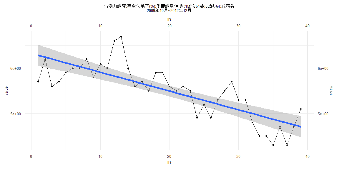
Call:
lm(formula = value ~ ID)

Residuals:
    Min      1Q  Median      3Q     Max
-0.6017 -0.2072 -0.0354  0.2135  0.9141

Coefficients:
             Estimate Std. Error t value             Pr(>|t|)
(Intercept)  6.326451   0.119532  52.927 < 0.0000000000000002 ***
ID          -0.041579   0.005209  -7.983        0.00000000145 ***
---
Signif. codes:  0 '***' 0.001 '**' 0.01 '*' 0.05 '.' 0.1 ' ' 1

Residual standard error: 0.3661 on 37 degrees of freedom
Multiple R-squared:  0.6327,    Adjusted R-squared:  0.6227
F-statistic: 63.73 on 1 and 37 DF,  p-value: 0.000000001451


    Two-sample Kolmogorov-Smirnov test

data:  lm_residuals and rnorm(n = length(lm_residuals), mean = 0, sd = sd(lm_residuals))
D = 0.15385, p-value = 0.7523
alternative hypothesis: two-sided


    Durbin-Watson test

data:  value ~ ID
DW = 0.86632, p-value = 0.00001975
alternative hypothesis: true autocorrelation is greater than 0


    studentized Breusch-Pagan test

data:  value ~ ID
BP = 0.1661, df = 1, p-value = 0.6836


    Box-Ljung test

data:  lm_residuals
X-squared = 11.23, df = 1, p-value = 0.0008049
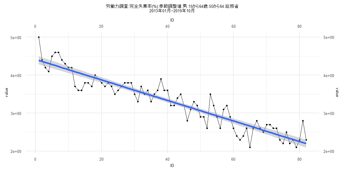
Call:
lm(formula = value ~ ID)

Residuals:
     Min       1Q   Median       3Q      Max
-0.55866 -0.16011 -0.00468  0.15552  0.61131

Coefficients:
             Estimate Std. Error t value            Pr(>|t|)
(Intercept)  4.415718   0.054585   80.90 <0.0000000000000002 ***
ID          -0.027032   0.001143  -23.66 <0.0000000000000002 ***
---
Signif. codes:  0 '***' 0.001 '**' 0.01 '*' 0.05 '.' 0.1 ' ' 1

Residual standard error: 0.2449 on 80 degrees of freedom
Multiple R-squared:  0.875, Adjusted R-squared:  0.8734
F-statistic: 559.8 on 1 and 80 DF,  p-value: < 0.00000000000000022


    Two-sample Kolmogorov-Smirnov test

data:  lm_residuals and rnorm(n = length(lm_residuals), mean = 0, sd = sd(lm_residuals))
D = 0.097561, p-value = 0.8332
alternative hypothesis: two-sided


    Durbin-Watson test

data:  value ~ ID
DW = 1.1763, p-value = 0.00002718
alternative hypothesis: true autocorrelation is greater than 0


    studentized Breusch-Pagan test

data:  value ~ ID
BP = 0.10363, df = 1, p-value = 0.7475


    Box-Ljung test

data:  lm_residuals
X-squared = 11.759, df = 1, p-value = 0.0006054
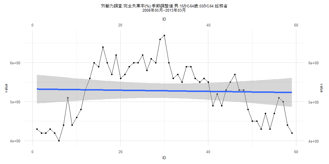
Call:
lm(formula = value ~ ID)

Residuals:
    Min      1Q  Median      3Q     Max
-1.3171 -0.6291  0.2246  0.6015  1.4186

Coefficients:
            Estimate Std. Error t value            Pr(>|t|)
(Intercept)  5.32607    0.18937  28.124 <0.0000000000000002 ***
ID          -0.00149    0.00549  -0.271               0.787
---
Signif. codes:  0 '***' 0.001 '**' 0.01 '*' 0.05 '.' 0.1 ' ' 1

Residual standard error: 0.7181 on 57 degrees of freedom
Multiple R-squared:  0.001291,  Adjusted R-squared:  -0.01623
F-statistic: 0.0737 on 1 and 57 DF,  p-value: 0.787


    Two-sample Kolmogorov-Smirnov test

data:  lm_residuals and rnorm(n = length(lm_residuals), mean = 0, sd = sd(lm_residuals))
D = 0.11864, p-value = 0.8052
alternative hypothesis: two-sided


    Durbin-Watson test

data:  value ~ ID
DW = 0.23782, p-value < 0.00000000000000022
alternative hypothesis: true autocorrelation is greater than 0


    studentized Breusch-Pagan test

data:  value ~ ID
BP = 7.3451, df = 1, p-value = 0.006724


    Box-Ljung test

data:  lm_residuals
X-squared = 44.296, df = 1, p-value = 0.00000000002823
Call:
lm(formula = value ~ ID)

Residuals:
     Min       1Q   Median       3Q      Max
-0.56385 -0.16009  0.00267  0.15867  0.56015

Coefficients:
             Estimate Std. Error t value            Pr(>|t|)
(Intercept)  4.306816   0.054238   79.41 <0.0000000000000002 ***
ID          -0.026500   0.001178  -22.50 <0.0000000000000002 ***
---
Signif. codes:  0 '***' 0.001 '**' 0.01 '*' 0.05 '.' 0.1 ' ' 1

Residual standard error: 0.2388 on 77 degrees of freedom
Multiple R-squared:  0.8679,    Adjusted R-squared:  0.8662
F-statistic: 506.1 on 1 and 77 DF,  p-value: < 0.00000000000000022


    Two-sample Kolmogorov-Smirnov test

data:  lm_residuals and rnorm(n = length(lm_residuals), mean = 0, sd = sd(lm_residuals))
D = 0.10127, p-value = 0.8161
alternative hypothesis: two-sided


    Durbin-Watson test

data:  value ~ ID
DW = 1.2028, p-value = 0.00006381
alternative hypothesis: true autocorrelation is greater than 0


    studentized Breusch-Pagan test

data:  value ~ ID
BP = 0.054879, df = 1, p-value = 0.8148


    Box-Ljung test

data:  lm_residuals
X-squared = 12.739, df = 1, p-value = 0.0003581