Analysis
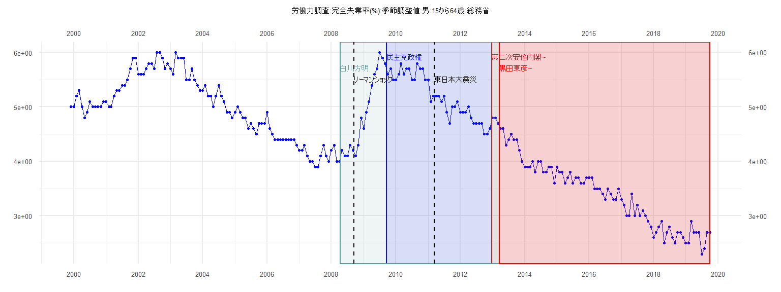
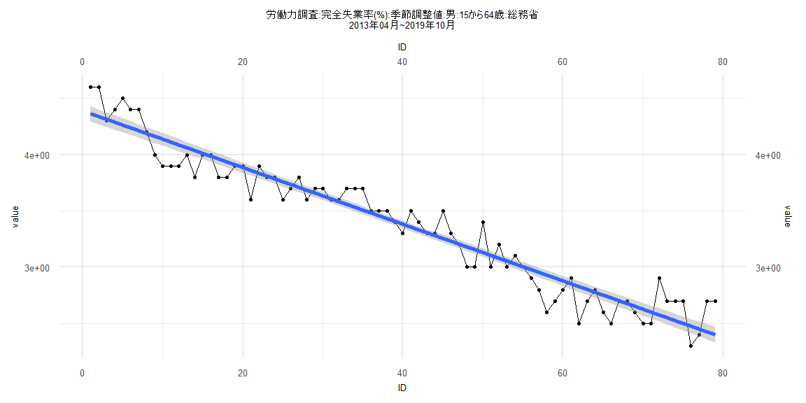
[1] "労働力調査:完全失業率(%):季節調整値:男:15から64歳:総務省"
     Jan Feb Mar Apr May Jun Jul Aug Sep Oct Nov Dec
1999                                             5.0
2000 5.0 5.2 5.3 5.0 4.8 4.9 5.1 5.0 5.0 5.0 5.0 5.1
2001 5.1 5.0 5.0 5.2 5.3 5.3 5.4 5.4 5.5 5.7 5.9 5.9
2002 5.6 5.6 5.6 5.7 5.8 5.8 5.7 6.0 6.0 5.9 5.7 5.8
2003 5.7 5.6 6.0 5.9 5.9 5.9 5.5 5.5 5.7 5.5 5.4 5.3
2004 5.3 5.4 5.2 5.2 5.0 5.2 5.4 5.2 5.1 4.9 4.9 4.8
2005 4.9 5.0 4.9 4.8 4.8 4.6 4.7 4.6 4.5 4.7 4.7 4.7
2006 4.9 4.6 4.5 4.4 4.4 4.4 4.4 4.4 4.4 4.4 4.4 4.3
2007 4.2 4.2 4.3 4.1 4.0 4.0 3.9 3.9 4.1 4.3 4.1 4.0
2008 4.2 4.3 4.0 4.0 4.2 4.1 4.1 4.3 4.2 4.1 4.3 4.8
2009 4.6 4.9 5.1 5.4 5.6 5.7 6.0 5.9 5.8 5.6 5.7 5.5
2010 5.5 5.6 5.8 5.6 5.7 5.7 5.5 5.5 5.8 5.7 5.7 5.5
2011 5.5 5.1 5.2 5.2 5.2 5.1 5.2 4.9 4.7 5.0 5.0 5.1
2012 4.9 4.9 4.9 5.0 4.8 4.7 4.7 4.7 4.7 4.5 4.5 4.6
2013 4.8 4.8 4.7 4.6 4.6 4.3 4.4 4.5 4.4 4.4 4.2 4.0
2014 3.9 3.9 3.9 4.0 3.8 4.0 4.0 3.8 3.8 3.9 3.9 3.6
2015 3.9 3.8 3.8 3.6 3.7 3.8 3.6 3.7 3.7 3.6 3.6 3.7
2016 3.7 3.7 3.5 3.5 3.5 3.4 3.3 3.5 3.4 3.3 3.3 3.5
2017 3.3 3.2 3.0 3.0 3.4 3.0 3.2 3.0 3.1 3.0 2.9 2.8
2018 2.6 2.7 2.8 2.9 2.5 2.7 2.8 2.6 2.5 2.7 2.7 2.6
2019 2.5 2.5 2.9 2.7 2.7 2.7 2.3 2.4 2.7 2.7
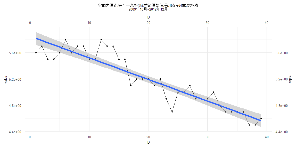
Call:
lm(formula = value ~ ID)

Residuals:
     Min       1Q   Median       3Q      Max
-0.36040 -0.07475  0.00233  0.09281  0.34389

Coefficients:
             Estimate Std. Error t value            Pr(>|t|)
(Intercept)  5.851822   0.050239  116.48 <0.0000000000000002 ***
ID          -0.032976   0.002189  -15.06 <0.0000000000000002 ***
---
Signif. codes:  0 '***' 0.001 '**' 0.01 '*' 0.05 '.' 0.1 ' ' 1

Residual standard error: 0.1539 on 37 degrees of freedom
Multiple R-squared:  0.8598,    Adjusted R-squared:  0.856
F-statistic: 226.9 on 1 and 37 DF,  p-value: < 0.00000000000000022


    Two-sample Kolmogorov-Smirnov test

data:  lm_residuals and rnorm(n = length(lm_residuals), mean = 0, sd = sd(lm_residuals))
D = 0.20513, p-value = 0.3888
alternative hypothesis: two-sided


    Durbin-Watson test

data:  value ~ ID
DW = 0.99934, p-value = 0.0001816
alternative hypothesis: true autocorrelation is greater than 0


    studentized Breusch-Pagan test

data:  value ~ ID
BP = 3.6548, df = 1, p-value = 0.05591


    Box-Ljung test

data:  lm_residuals
X-squared = 9.3874, df = 1, p-value = 0.002185
Call:
lm(formula = value ~ ID)

Residuals:
     Min       1Q   Median       3Q      Max
-0.32312 -0.10337 -0.01212  0.10843  0.34203

Coefficients:
              Estimate Std. Error t value            Pr(>|t|)
(Intercept)  4.5140921  0.0363420  124.21 <0.0000000000000002 ***
ID          -0.0260816  0.0007607  -34.29 <0.0000000000000002 ***
---
Signif. codes:  0 '***' 0.001 '**' 0.01 '*' 0.05 '.' 0.1 ' ' 1

Residual standard error: 0.163 on 80 degrees of freedom
Multiple R-squared:  0.9363,    Adjusted R-squared:  0.9355
F-statistic:  1176 on 1 and 80 DF,  p-value: < 0.00000000000000022


    Two-sample Kolmogorov-Smirnov test

data:  lm_residuals and rnorm(n = length(lm_residuals), mean = 0, sd = sd(lm_residuals))
D = 0.097561, p-value = 0.8332
alternative hypothesis: two-sided


    Durbin-Watson test

data:  value ~ ID
DW = 1.023, p-value = 0.0000005737
alternative hypothesis: true autocorrelation is greater than 0


    studentized Breusch-Pagan test

data:  value ~ ID
BP = 0.054772, df = 1, p-value = 0.815


    Box-Ljung test

data:  lm_residuals
X-squared = 16.526, df = 1, p-value = 0.00004799
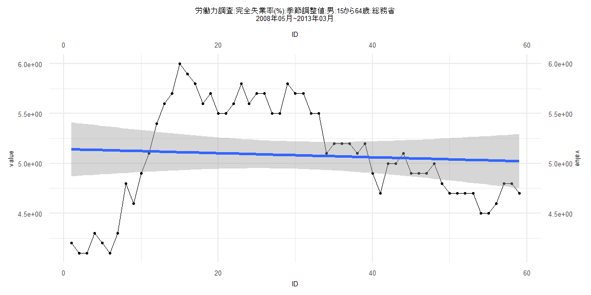
Call:
lm(formula = value ~ ID)

Residuals:
     Min       1Q   Median       3Q      Max
-1.04065 -0.33676 -0.02214  0.45255  0.88609

Coefficients:
             Estimate Std. Error t value            Pr(>|t|)
(Intercept)  5.144769   0.138631  37.111 <0.0000000000000002 ***
ID          -0.002057   0.004019  -0.512               0.611
---
Signif. codes:  0 '***' 0.001 '**' 0.01 '*' 0.05 '.' 0.1 ' ' 1

Residual standard error: 0.5257 on 57 degrees of freedom
Multiple R-squared:  0.004577,  Adjusted R-squared:  -0.01289
F-statistic: 0.2621 on 1 and 57 DF,  p-value: 0.6107


    Two-sample Kolmogorov-Smirnov test

data:  lm_residuals and rnorm(n = length(lm_residuals), mean = 0, sd = sd(lm_residuals))
D = 0.13559, p-value = 0.6544
alternative hypothesis: two-sided


    Durbin-Watson test

data:  value ~ ID
DW = 0.11252, p-value < 0.00000000000000022
alternative hypothesis: true autocorrelation is greater than 0


    studentized Breusch-Pagan test

data:  value ~ ID
BP = 25.502, df = 1, p-value = 0.0000004419


    Box-Ljung test

data:  lm_residuals
X-squared = 51.635, df = 1, p-value = 0.0000000000006686
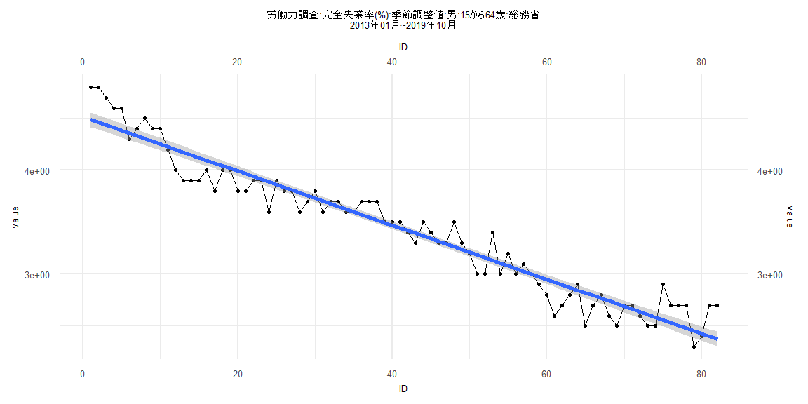
Call:
lm(formula = value ~ ID)

Residuals:
     Min       1Q   Median       3Q      Max
-0.32799 -0.10316 -0.00349  0.08157  0.32436

Coefficients:
              Estimate Std. Error t value            Pr(>|t|)
(Intercept)  4.3877313  0.0347366  126.31 <0.0000000000000002 ***
ID          -0.0251680  0.0007544  -33.36 <0.0000000000000002 ***
---
Signif. codes:  0 '***' 0.001 '**' 0.01 '*' 0.05 '.' 0.1 ' ' 1

Residual standard error: 0.1529 on 77 degrees of freedom
Multiple R-squared:  0.9353,    Adjusted R-squared:  0.9344
F-statistic:  1113 on 1 and 77 DF,  p-value: < 0.00000000000000022


    Two-sample Kolmogorov-Smirnov test

data:  lm_residuals and rnorm(n = length(lm_residuals), mean = 0, sd = sd(lm_residuals))
D = 0.10127, p-value = 0.8161
alternative hypothesis: two-sided


    Durbin-Watson test

data:  value ~ ID
DW = 1.2019, p-value = 0.0000626
alternative hypothesis: true autocorrelation is greater than 0


    studentized Breusch-Pagan test

data:  value ~ ID
BP = 1.0457, df = 1, p-value = 0.3065


    Box-Ljung test

data:  lm_residuals
X-squared = 10.534, df = 1, p-value = 0.001172