Analysis
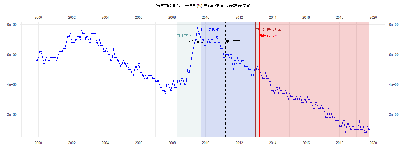
[1] "労働力調査:完全失業率(%):季節調整値:男:総数:総務省"
     Jan Feb Mar Apr May Jun Jul Aug Sep Oct Nov Dec
1999                                             4.8
2000 4.9 5.1 5.1 4.9 4.7 4.8 4.9 4.8 4.8 4.9 4.9 4.9
2001 4.9 4.8 4.9 5.1 5.1 5.1 5.2 5.2 5.4 5.6 5.6 5.7
2002 5.4 5.4 5.4 5.5 5.6 5.6 5.5 5.8 5.7 5.7 5.5 5.6
2003 5.5 5.4 5.7 5.7 5.7 5.7 5.4 5.3 5.5 5.3 5.3 5.1
2004 5.1 5.2 5.0 5.0 4.8 4.9 5.2 4.9 4.9 4.8 4.7 4.6
2005 4.7 4.8 4.7 4.6 4.7 4.5 4.5 4.4 4.3 4.5 4.6 4.5
2006 4.7 4.4 4.4 4.3 4.2 4.3 4.2 4.3 4.3 4.3 4.2 4.2
2007 4.1 4.1 4.1 4.0 3.9 3.8 3.8 3.7 4.0 4.0 3.9 3.8
2008 4.0 4.1 3.9 3.9 4.1 4.1 4.0 4.2 4.1 4.0 4.1 4.5
2009 4.4 4.6 4.9 5.2 5.4 5.5 5.9 5.7 5.6 5.4 5.5 5.3
2010 5.3 5.4 5.5 5.4 5.5 5.5 5.4 5.4 5.6 5.4 5.4 5.2
2011 5.2 4.9 5.0 5.0 5.0 4.9 5.0 4.7 4.5 4.8 4.7 4.9
2012 4.7 4.7 4.8 4.8 4.6 4.6 4.6 4.5 4.5 4.3 4.3 4.5
2013 4.5 4.6 4.5 4.4 4.3 4.2 4.2 4.4 4.2 4.2 4.1 3.8
2014 3.8 3.7 3.8 3.9 3.7 3.9 3.8 3.7 3.7 3.8 3.7 3.5
2015 3.7 3.6 3.6 3.5 3.5 3.6 3.5 3.5 3.6 3.4 3.4 3.5
2016 3.4 3.6 3.5 3.4 3.4 3.2 3.2 3.4 3.3 3.2 3.2 3.3
2017 3.2 3.1 2.9 2.9 3.2 2.9 3.0 2.9 2.9 2.8 2.8 2.8
2018 2.6 2.6 2.7 2.8 2.4 2.6 2.7 2.6 2.5 2.6 2.6 2.5
2019 2.5 2.5 2.8 2.5 2.5 2.6 2.4 2.4 2.6 2.5
Call:
lm(formula = value ~ ID)

Residuals:
     Min       1Q   Median       3Q      Max
-0.36583 -0.06403 -0.00336  0.09998  0.35474

Coefficients:
             Estimate Std. Error t value            Pr(>|t|)
(Intercept)  5.624696   0.047064  119.51 <0.0000000000000002 ***
ID          -0.031619   0.002051  -15.42 <0.0000000000000002 ***
---
Signif. codes:  0 '***' 0.001 '**' 0.01 '*' 0.05 '.' 0.1 ' ' 1

Residual standard error: 0.1441 on 37 degrees of freedom
Multiple R-squared:  0.8653,    Adjusted R-squared:  0.8617
F-statistic: 237.7 on 1 and 37 DF,  p-value: < 0.00000000000000022


    Two-sample Kolmogorov-Smirnov test

data:  lm_residuals and rnorm(n = length(lm_residuals), mean = 0, sd = sd(lm_residuals))
D = 0.20513, p-value = 0.3888
alternative hypothesis: two-sided


    Durbin-Watson test

data:  value ~ ID
DW = 1.003, p-value = 0.000192
alternative hypothesis: true autocorrelation is greater than 0


    studentized Breusch-Pagan test

data:  value ~ ID
BP = 1.5371, df = 1, p-value = 0.215


    Box-Ljung test

data:  lm_residuals
X-squared = 9.1604, df = 1, p-value = 0.002473
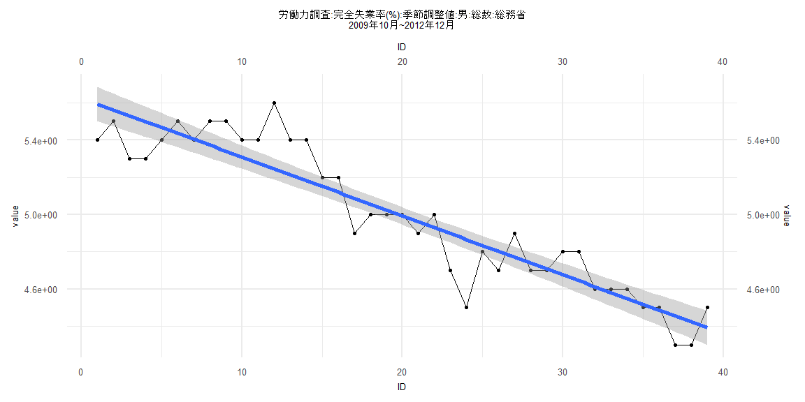
Call:
lm(formula = value ~ ID)

Residuals:
     Min       1Q   Median       3Q      Max
-0.32364 -0.08642 -0.00123  0.07969  0.32469

Coefficients:
              Estimate Std. Error t value            Pr(>|t|)
(Intercept)  4.3245709  0.0306336  141.17 <0.0000000000000002 ***
ID          -0.0246297  0.0006412  -38.41 <0.0000000000000002 ***
---
Signif. codes:  0 '***' 0.001 '**' 0.01 '*' 0.05 '.' 0.1 ' ' 1

Residual standard error: 0.1374 on 80 degrees of freedom
Multiple R-squared:  0.9486,    Adjusted R-squared:  0.9479
F-statistic:  1475 on 1 and 80 DF,  p-value: < 0.00000000000000022


    Two-sample Kolmogorov-Smirnov test

data:  lm_residuals and rnorm(n = length(lm_residuals), mean = 0, sd = sd(lm_residuals))
D = 0.097561, p-value = 0.8332
alternative hypothesis: two-sided


    Durbin-Watson test

data:  value ~ ID
DW = 1.0262, p-value = 0.0000006279
alternative hypothesis: true autocorrelation is greater than 0


    studentized Breusch-Pagan test

data:  value ~ ID
BP = 1.1262, df = 1, p-value = 0.2886


    Box-Ljung test

data:  lm_residuals
X-squared = 18.077, df = 1, p-value = 0.00002121
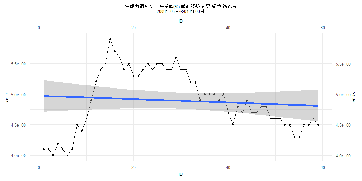
Call:
lm(formula = value ~ ID)

Residuals:
     Min       1Q   Median       3Q      Max
-0.96601 -0.32394 -0.04187  0.48089  0.96710

Coefficients:
             Estimate Std. Error t value            Pr(>|t|)
(Intercept)  4.974284   0.132165   37.64 <0.0000000000000002 ***
ID          -0.002759   0.003831   -0.72               0.474
---
Signif. codes:  0 '***' 0.001 '**' 0.01 '*' 0.05 '.' 0.1 ' ' 1

Residual standard error: 0.5011 on 57 degrees of freedom
Multiple R-squared:  0.009014,  Adjusted R-squared:  -0.008372
F-statistic: 0.5184 on 1 and 57 DF,  p-value: 0.4744


    Two-sample Kolmogorov-Smirnov test

data:  lm_residuals and rnorm(n = length(lm_residuals), mean = 0, sd = sd(lm_residuals))
D = 0.10169, p-value = 0.9239
alternative hypothesis: two-sided


    Durbin-Watson test

data:  value ~ ID
DW = 0.11055, p-value < 0.00000000000000022
alternative hypothesis: true autocorrelation is greater than 0


    studentized Breusch-Pagan test

data:  value ~ ID
BP = 27.018, df = 1, p-value = 0.0000002015


    Box-Ljung test

data:  lm_residuals
X-squared = 51.929, df = 1, p-value = 0.0000000000005754
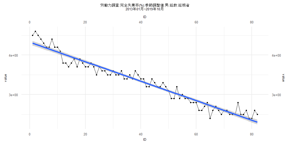
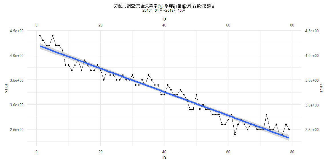
Call:
lm(formula = value ~ ID)

Residuals:
     Min       1Q   Median       3Q      Max
-0.33081 -0.07904  0.00013  0.07907  0.30926

Coefficients:
             Estimate Std. Error t value            Pr(>|t|)
(Intercept)  4.210029   0.029191  144.22 <0.0000000000000002 ***
ID          -0.023858   0.000634  -37.63 <0.0000000000000002 ***
---
Signif. codes:  0 '***' 0.001 '**' 0.01 '*' 0.05 '.' 0.1 ' ' 1

Residual standard error: 0.1285 on 77 degrees of freedom
Multiple R-squared:  0.9484,    Adjusted R-squared:  0.9478
F-statistic:  1416 on 1 and 77 DF,  p-value: < 0.00000000000000022


    Two-sample Kolmogorov-Smirnov test

data:  lm_residuals and rnorm(n = length(lm_residuals), mean = 0, sd = sd(lm_residuals))
D = 0.075949, p-value = 0.978
alternative hypothesis: two-sided


    Durbin-Watson test

data:  value ~ ID
DW = 1.1985, p-value = 0.00005837
alternative hypothesis: true autocorrelation is greater than 0


    studentized Breusch-Pagan test

data:  value ~ ID
BP = 0.028303, df = 1, p-value = 0.8664


    Box-Ljung test

data:  lm_residuals
X-squared = 11.278, df = 1, p-value = 0.0007845