Analysis
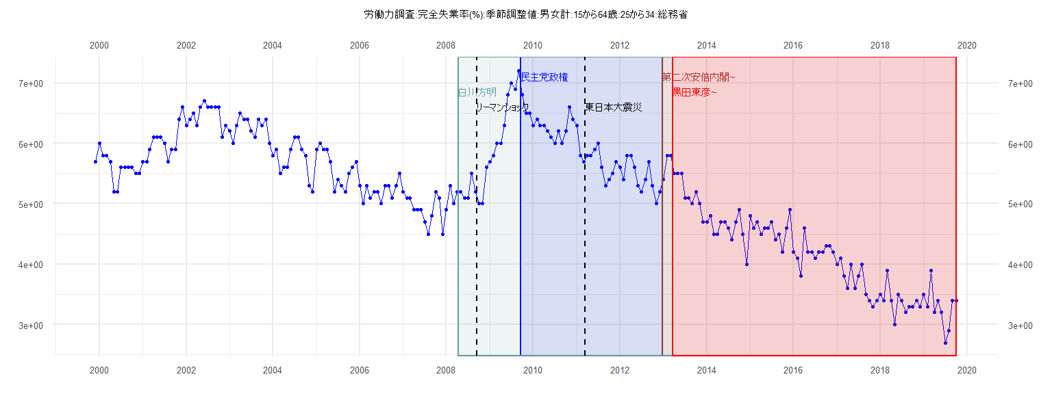
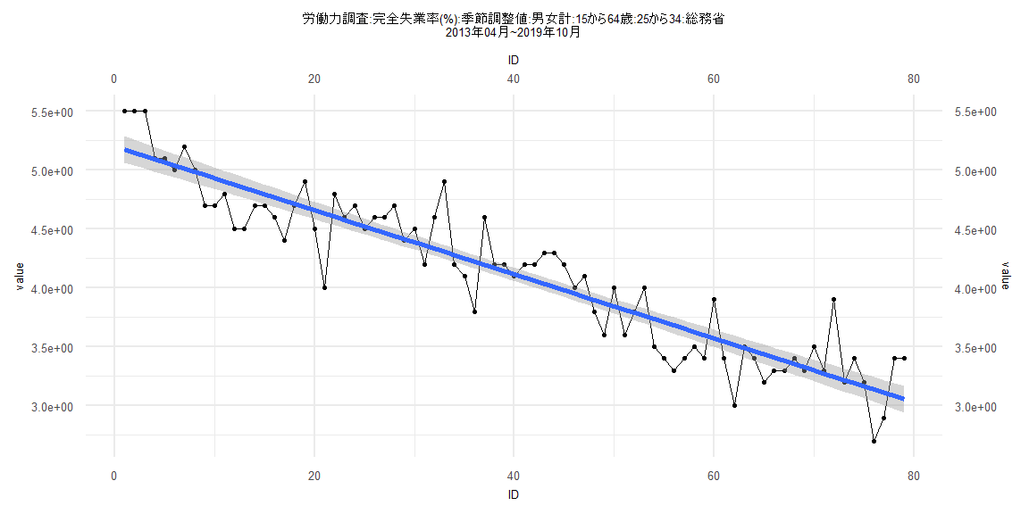
[1] "労働力調査:完全失業率(%):季節調整値:男女計:15から64歳:25から34:総務省"
     Jan Feb Mar Apr May Jun Jul Aug Sep Oct Nov Dec
1999                                             5.7
2000 6.0 5.8 5.8 5.7 5.2 5.2 5.6 5.6 5.6 5.6 5.5 5.5
2001 5.7 5.7 5.9 6.1 6.1 6.1 6.0 5.7 5.9 5.9 6.4 6.6
2002 6.3 6.4 6.5 6.3 6.6 6.7 6.6 6.6 6.6 6.6 6.1 6.3
2003 6.2 6.0 6.3 6.5 6.4 6.4 6.2 6.1 6.4 6.3 6.4 6.0
2004 5.8 5.9 5.5 5.6 5.6 5.9 6.1 6.1 5.9 5.8 5.3 5.2
2005 5.9 6.0 5.9 5.9 5.7 5.2 5.4 5.3 5.2 5.5 5.6 5.7
2006 5.3 5.0 5.3 5.1 5.2 5.2 5.0 5.3 5.3 5.1 5.3 5.5
2007 5.2 5.1 5.1 4.9 4.9 4.9 4.7 4.5 4.8 5.2 5.1 4.5
2008 4.9 5.3 5.0 5.2 5.2 5.1 5.1 5.5 5.2 5.0 5.0 5.6
2009 5.7 5.8 6.0 6.0 6.3 6.8 7.0 6.9 7.2 6.8 6.5 6.5
2010 6.3 6.4 6.3 6.3 6.2 6.1 6.0 6.2 6.0 6.2 6.6 6.4
2011 6.3 5.8 5.7 5.8 5.8 5.9 6.0 5.6 5.3 5.4 5.5 5.7
2012 5.6 5.4 5.8 5.8 5.6 5.3 5.2 5.4 5.7 5.3 5.0 5.2
2013 5.4 5.8 5.8 5.5 5.5 5.5 5.1 5.1 5.0 5.2 5.0 4.7
2014 4.7 4.8 4.5 4.5 4.7 4.7 4.6 4.4 4.7 4.9 4.5 4.0
2015 4.8 4.6 4.7 4.5 4.6 4.6 4.7 4.4 4.5 4.2 4.6 4.9
2016 4.2 4.1 3.8 4.6 4.2 4.2 4.1 4.2 4.2 4.3 4.3 4.2
2017 4.0 4.1 3.8 3.6 4.0 3.6 3.8 4.0 3.5 3.4 3.3 3.4
2018 3.5 3.4 3.9 3.4 3.0 3.5 3.4 3.2 3.3 3.3 3.4 3.3
2019 3.5 3.3 3.9 3.2 3.4 3.2 2.7 2.9 3.4 3.4
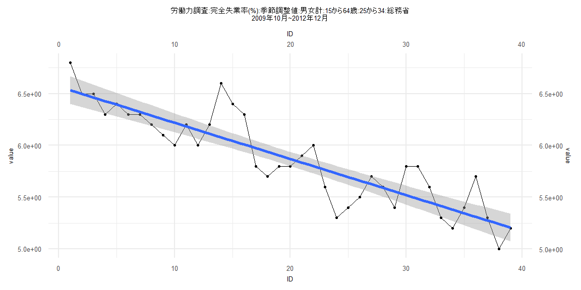
Call:
lm(formula = value ~ ID)

Residuals:
     Min       1Q   Median       3Q      Max
-0.42939 -0.15419 -0.00500  0.08077  0.52101

Coefficients:
             Estimate Std. Error t value             Pr(>|t|)
(Intercept)  6.568421   0.068859   95.39 < 0.0000000000000002 ***
ID          -0.034960   0.003001  -11.65   0.0000000000000608 ***
---
Signif. codes:  0 '***' 0.001 '**' 0.01 '*' 0.05 '.' 0.1 ' ' 1

Residual standard error: 0.2109 on 37 degrees of freedom
Multiple R-squared:  0.7858,    Adjusted R-squared:   0.78
F-statistic: 135.8 on 1 and 37 DF,  p-value: 0.00000000000006077


    Two-sample Kolmogorov-Smirnov test

data:  lm_residuals and rnorm(n = length(lm_residuals), mean = 0, sd = sd(lm_residuals))
D = 0.25641, p-value = 0.1547
alternative hypothesis: two-sided


    Durbin-Watson test

data:  value ~ ID
DW = 1.1027, p-value = 0.0007677
alternative hypothesis: true autocorrelation is greater than 0


    studentized Breusch-Pagan test

data:  value ~ ID
BP = 0.37138, df = 1, p-value = 0.5423


    Box-Ljung test

data:  lm_residuals
X-squared = 7.6742, df = 1, p-value = 0.005602
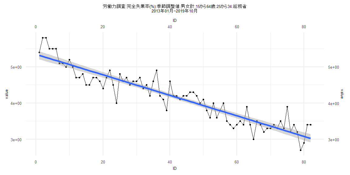
Call:
lm(formula = value ~ ID)

Residuals:
     Min       1Q   Median       3Q      Max
-0.66683 -0.18014 -0.00986  0.16668  0.67539

Coefficients:
             Estimate Std. Error t value            Pr(>|t|)
(Intercept)  5.345528   0.057948   92.25 <0.0000000000000002 ***
ID          -0.028279   0.001213  -23.32 <0.0000000000000002 ***
---
Signif. codes:  0 '***' 0.001 '**' 0.01 '*' 0.05 '.' 0.1 ' ' 1

Residual standard error: 0.26 on 80 degrees of freedom
Multiple R-squared:  0.8717,    Adjusted R-squared:  0.8701
F-statistic: 543.6 on 1 and 80 DF,  p-value: < 0.00000000000000022


    Two-sample Kolmogorov-Smirnov test

data:  lm_residuals and rnorm(n = length(lm_residuals), mean = 0, sd = sd(lm_residuals))
D = 0.097561, p-value = 0.8332
alternative hypothesis: two-sided


    Durbin-Watson test

data:  value ~ ID
DW = 1.3523, p-value = 0.0008407
alternative hypothesis: true autocorrelation is greater than 0


    studentized Breusch-Pagan test

data:  value ~ ID
BP = 0.12552, df = 1, p-value = 0.7231


    Box-Ljung test

data:  lm_residuals
X-squared = 8.1895, df = 1, p-value = 0.004213
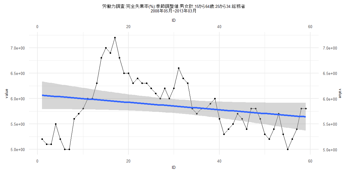
Call:
lm(formula = value ~ ID)

Residuals:
     Min       1Q   Median       3Q      Max
-1.02830 -0.35002  0.00832  0.34013  1.25226

Coefficients:
             Estimate Std. Error t value            Pr(>|t|)
(Intercept)  6.072238   0.139766  43.446 <0.0000000000000002 ***
ID          -0.007323   0.004052  -1.807               0.076 .
---
Signif. codes:  0 '***' 0.001 '**' 0.01 '*' 0.05 '.' 0.1 ' ' 1

Residual standard error: 0.53 on 57 degrees of freedom
Multiple R-squared:  0.05421,   Adjusted R-squared:  0.03762
F-statistic: 3.267 on 1 and 57 DF,  p-value: 0.07596


    Two-sample Kolmogorov-Smirnov test

data:  lm_residuals and rnorm(n = length(lm_residuals), mean = 0, sd = sd(lm_residuals))
D = 0.11864, p-value = 0.8052
alternative hypothesis: two-sided


    Durbin-Watson test

data:  value ~ ID
DW = 0.21562, p-value < 0.00000000000000022
alternative hypothesis: true autocorrelation is greater than 0


    studentized Breusch-Pagan test

data:  value ~ ID
BP = 17.174, df = 1, p-value = 0.00003411


    Box-Ljung test

data:  lm_residuals
X-squared = 46.755, df = 1, p-value = 0.000000000008046
Call:
lm(formula = value ~ ID)

Residuals:
     Min       1Q   Median       3Q      Max
-0.63121 -0.15900  0.00708  0.18174  0.65390

Coefficients:
             Estimate Std. Error t value            Pr(>|t|)
(Intercept)  5.201558   0.056602   91.90 <0.0000000000000002 ***
ID          -0.027159   0.001229  -22.09 <0.0000000000000002 ***
---
Signif. codes:  0 '***' 0.001 '**' 0.01 '*' 0.05 '.' 0.1 ' ' 1

Residual standard error: 0.2492 on 77 degrees of freedom
Multiple R-squared:  0.8637,    Adjusted R-squared:  0.862
F-statistic: 488.1 on 1 and 77 DF,  p-value: < 0.00000000000000022


    Two-sample Kolmogorov-Smirnov test

data:  lm_residuals and rnorm(n = length(lm_residuals), mean = 0, sd = sd(lm_residuals))
D = 0.088608, p-value = 0.9184
alternative hypothesis: two-sided


    Durbin-Watson test

data:  value ~ ID
DW = 1.4755, p-value = 0.006222
alternative hypothesis: true autocorrelation is greater than 0


    studentized Breusch-Pagan test

data:  value ~ ID
BP = 0.17508, df = 1, p-value = 0.6756


    Box-Ljung test

data:  lm_residuals
X-squared = 4.6767, df = 1, p-value = 0.03057