Analysis
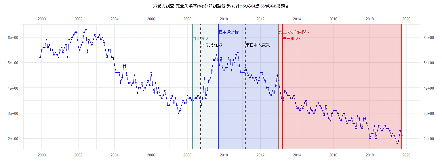
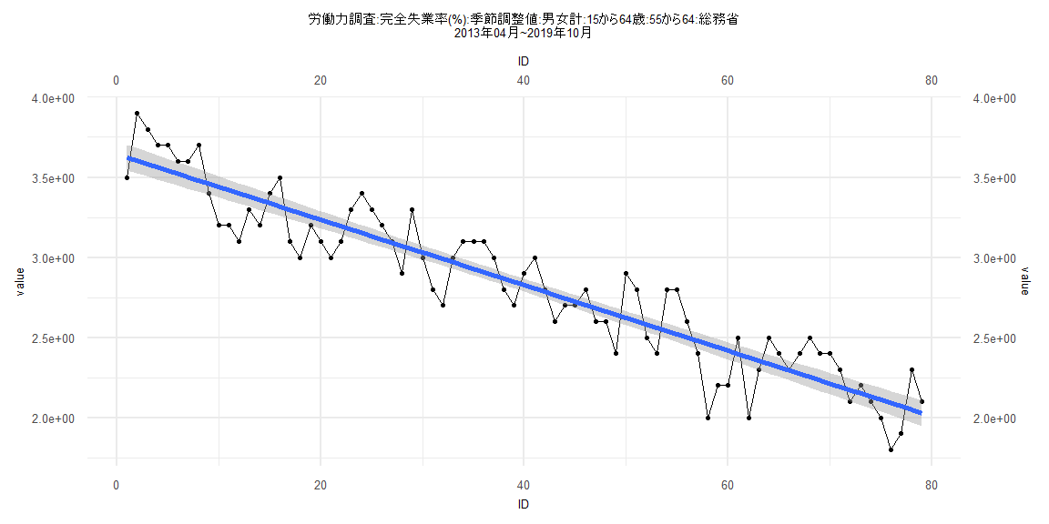
[1] "労働力調査:完全失業率(%):季節調整値:男女計:15から64歳:55から64:総務省"
     Jan Feb Mar Apr May Jun Jul Aug Sep Oct Nov Dec
1999                                             5.2
2000 5.5 5.6 5.6 5.9 5.6 5.7 5.5 5.5 5.3 5.4 5.3 5.2
2001 5.5 5.6 5.4 5.6 5.7 5.2 5.9 5.8 6.0 6.1 6.2 6.2
2002 5.6 5.5 5.7 5.8 6.2 6.3 5.4 5.9 5.8 5.7 5.9 6.1
2003 5.9 6.0 6.1 5.9 6.0 5.8 5.5 5.2 5.5 5.5 5.2 5.2
2004 4.9 4.6 4.6 4.6 4.2 4.4 4.9 4.9 4.5 4.2 4.2 4.1
2005 4.2 4.5 4.2 3.8 4.0 4.0 4.2 3.9 4.0 4.1 4.3 4.1
2006 4.6 4.1 3.8 4.2 3.8 4.0 3.7 3.6 3.7 3.9 3.6 3.3
2007 3.3 3.6 3.7 3.4 3.6 3.3 3.0 3.1 3.3 3.5 3.4 3.4
2008 3.7 3.6 3.6 3.5 3.5 3.6 3.6 3.7 3.6 3.3 3.6 4.4
2009 3.6 3.9 4.3 4.4 4.7 5.1 5.1 5.3 5.1 4.9 5.2 4.8
2010 4.7 4.8 4.8 5.2 5.1 4.7 5.1 5.0 5.3 5.4 4.9 4.6
2011 4.6 4.6 4.8 4.7 4.5 4.4 4.5 4.4 4.3 4.4 4.2 4.3
2012 4.6 4.6 4.4 4.3 4.0 4.0 3.8 3.7 3.9 3.8 4.1 4.5
2013 4.3 3.8 3.6 3.5 3.9 3.8 3.7 3.7 3.6 3.6 3.7 3.4
2014 3.2 3.2 3.1 3.3 3.2 3.4 3.5 3.1 3.0 3.2 3.1 3.0
2015 3.1 3.3 3.4 3.3 3.2 3.1 2.9 3.3 3.0 2.8 2.7 3.0
2016 3.1 3.1 3.1 3.0 2.8 2.7 2.9 3.0 2.8 2.6 2.7 2.7
2017 2.8 2.6 2.6 2.4 2.9 2.8 2.5 2.4 2.8 2.8 2.6 2.4
2018 2.0 2.2 2.2 2.5 2.0 2.3 2.5 2.4 2.3 2.4 2.5 2.4
2019 2.4 2.3 2.1 2.2 2.1 2.0 1.8 1.9 2.3 2.1
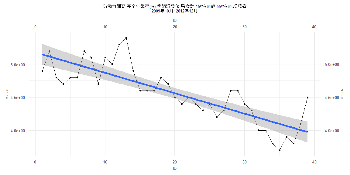
Call:
lm(formula = value ~ ID)

Residuals:
     Min       1Q   Median       3Q      Max
-0.39787 -0.18334 -0.05427  0.15663  0.62209

Coefficients:
             Estimate Std. Error t value             Pr(>|t|)
(Intercept)  5.179757   0.080915  64.015 < 0.0000000000000002 ***
ID          -0.030911   0.003526  -8.767       0.000000000146 ***
---
Signif. codes:  0 '***' 0.001 '**' 0.01 '*' 0.05 '.' 0.1 ' ' 1

Residual standard error: 0.2478 on 37 degrees of freedom
Multiple R-squared:  0.675, Adjusted R-squared:  0.6663
F-statistic: 76.86 on 1 and 37 DF,  p-value: 0.0000000001458


    Two-sample Kolmogorov-Smirnov test

data:  lm_residuals and rnorm(n = length(lm_residuals), mean = 0, sd = sd(lm_residuals))
D = 0.10256, p-value = 0.9885
alternative hypothesis: two-sided


    Durbin-Watson test

data:  value ~ ID
DW = 0.8765, p-value = 0.0000238
alternative hypothesis: true autocorrelation is greater than 0


    studentized Breusch-Pagan test

data:  value ~ ID
BP = 0.0041914, df = 1, p-value = 0.9484


    Box-Ljung test

data:  lm_residuals
X-squared = 9.992, df = 1, p-value = 0.001572
Call:
lm(formula = value ~ ID)

Residuals:
     Min       1Q   Median       3Q      Max
-0.45502 -0.15517  0.01071  0.13815  0.58087

Coefficients:
             Estimate Std. Error t value            Pr(>|t|)
(Intercept)  3.740199   0.042234   88.56 <0.0000000000000002 ***
ID          -0.021069   0.000884  -23.83 <0.0000000000000002 ***
---
Signif. codes:  0 '***' 0.001 '**' 0.01 '*' 0.05 '.' 0.1 ' ' 1

Residual standard error: 0.1895 on 80 degrees of freedom
Multiple R-squared:  0.8765,    Adjusted R-squared:  0.875
F-statistic:   568 on 1 and 80 DF,  p-value: < 0.00000000000000022


    Two-sample Kolmogorov-Smirnov test

data:  lm_residuals and rnorm(n = length(lm_residuals), mean = 0, sd = sd(lm_residuals))
D = 0.097561, p-value = 0.8332
alternative hypothesis: two-sided


    Durbin-Watson test

data:  value ~ ID
DW = 1.178, p-value = 0.00002824
alternative hypothesis: true autocorrelation is greater than 0


    studentized Breusch-Pagan test

data:  value ~ ID
BP = 0.75149, df = 1, p-value = 0.386


    Box-Ljung test

data:  lm_residuals
X-squared = 10.474, df = 1, p-value = 0.001211
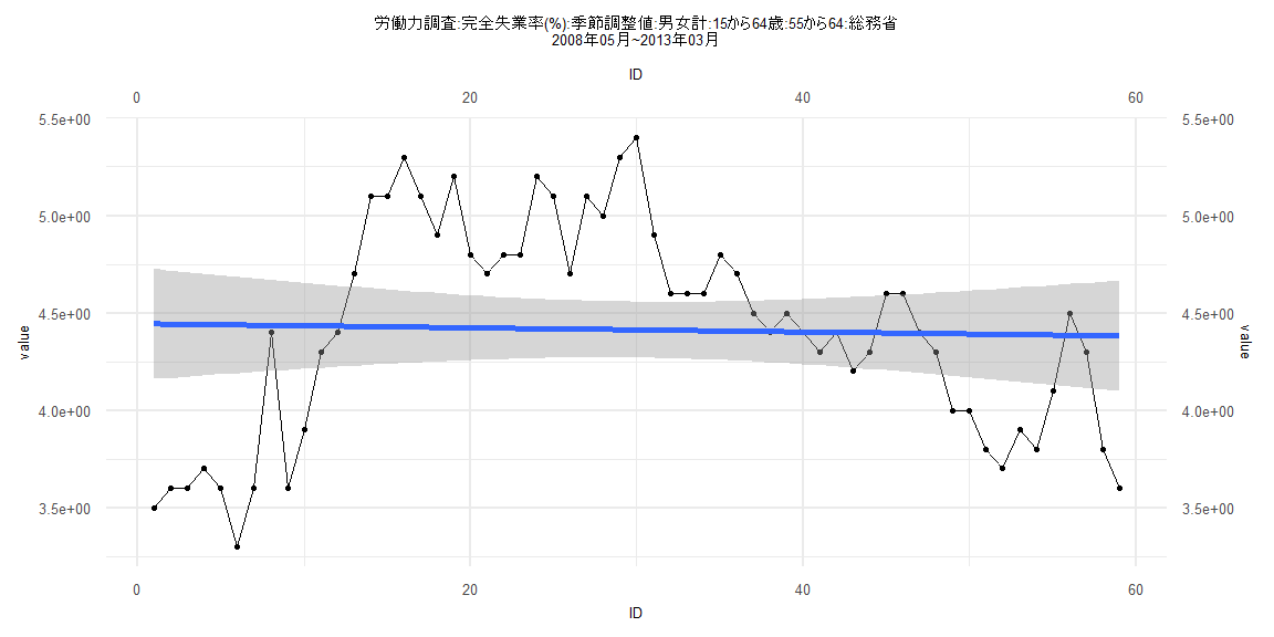
Call:
lm(formula = value ~ ID)

Residuals:
     Min       1Q   Median       3Q      Max
-1.13881 -0.44147  0.00432  0.37855  0.98644

Coefficients:
             Estimate Std. Error t value            Pr(>|t|)
(Intercept)  4.445120   0.145416   30.57 <0.0000000000000002 ***
ID          -0.001052   0.004215   -0.25               0.804
---
Signif. codes:  0 '***' 0.001 '**' 0.01 '*' 0.05 '.' 0.1 ' ' 1

Residual standard error: 0.5514 on 57 degrees of freedom
Multiple R-squared:  0.001091,  Adjusted R-squared:  -0.01643
F-statistic: 0.06228 on 1 and 57 DF,  p-value: 0.8038


    Two-sample Kolmogorov-Smirnov test

data:  lm_residuals and rnorm(n = length(lm_residuals), mean = 0, sd = sd(lm_residuals))
D = 0.15254, p-value = 0.5021
alternative hypothesis: two-sided


    Durbin-Watson test

data:  value ~ ID
DW = 0.25564, p-value < 0.00000000000000022
alternative hypothesis: true autocorrelation is greater than 0


    studentized Breusch-Pagan test

data:  value ~ ID
BP = 13.424, df = 1, p-value = 0.0002484


    Box-Ljung test

data:  lm_residuals
X-squared = 42.621, df = 1, p-value = 0.00000000006643
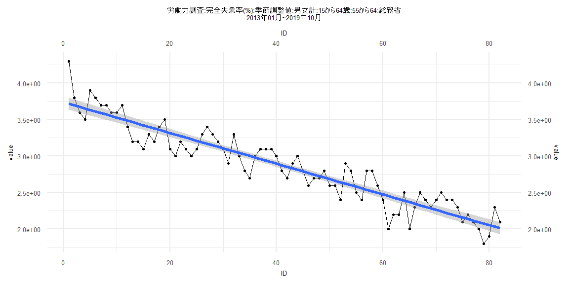
Call:
lm(formula = value ~ ID)

Residuals:
     Min       1Q   Median       3Q      Max
-0.45852 -0.14129  0.00759  0.15424  0.29640

Coefficients:
              Estimate Std. Error t value            Pr(>|t|)
(Intercept)  3.6444985  0.0409165   89.07 <0.0000000000000002 ***
ID          -0.0204479  0.0008886  -23.01 <0.0000000000000002 ***
---
Signif. codes:  0 '***' 0.001 '**' 0.01 '*' 0.05 '.' 0.1 ' ' 1

Residual standard error: 0.1801 on 77 degrees of freedom
Multiple R-squared:  0.873, Adjusted R-squared:  0.8714
F-statistic: 529.5 on 1 and 77 DF,  p-value: < 0.00000000000000022


    Two-sample Kolmogorov-Smirnov test

data:  lm_residuals and rnorm(n = length(lm_residuals), mean = 0, sd = sd(lm_residuals))
D = 0.12658, p-value = 0.5543
alternative hypothesis: two-sided


    Durbin-Watson test

data:  value ~ ID
DW = 1.2472, p-value = 0.000155
alternative hypothesis: true autocorrelation is greater than 0


    studentized Breusch-Pagan test

data:  value ~ ID
BP = 0.039121, df = 1, p-value = 0.8432


    Box-Ljung test

data:  lm_residuals
X-squared = 11.373, df = 1, p-value = 0.0007453