Analysis
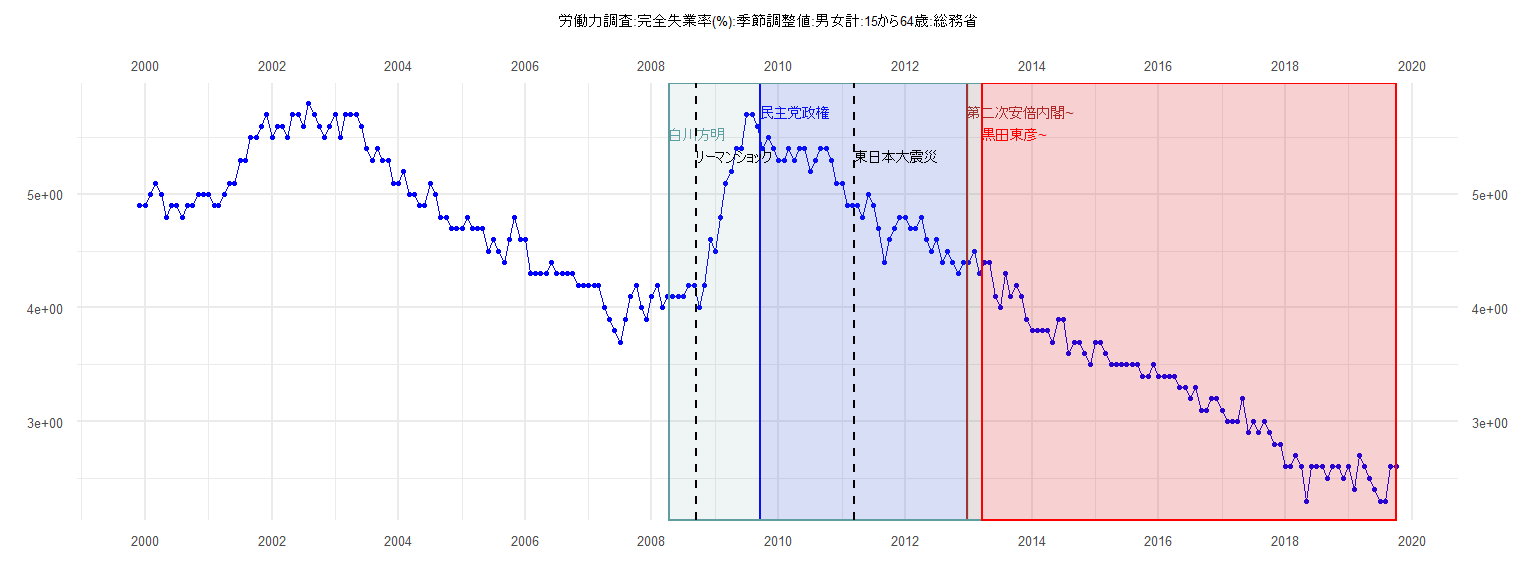
[1] "労働力調査:完全失業率(%):季節調整値:男女計:15から64歳:総務省"
     Jan Feb Mar Apr May Jun Jul Aug Sep Oct Nov Dec
1999                                             4.9
2000 4.9 5.0 5.1 5.0 4.8 4.9 4.9 4.8 4.9 4.9 5.0 5.0
2001 5.0 4.9 4.9 5.0 5.1 5.1 5.3 5.3 5.5 5.5 5.6 5.7
2002 5.5 5.6 5.6 5.5 5.7 5.7 5.6 5.8 5.7 5.6 5.5 5.6
2003 5.7 5.5 5.7 5.7 5.7 5.6 5.4 5.3 5.4 5.3 5.3 5.1
2004 5.1 5.2 5.0 5.0 4.9 4.9 5.1 5.0 4.8 4.8 4.7 4.7
2005 4.7 4.8 4.7 4.7 4.7 4.5 4.6 4.5 4.4 4.6 4.8 4.6
2006 4.6 4.3 4.3 4.3 4.3 4.4 4.3 4.3 4.3 4.3 4.2 4.2
2007 4.2 4.2 4.2 4.0 3.9 3.8 3.7 3.9 4.1 4.2 4.0 3.9
2008 4.1 4.2 4.0 4.1 4.1 4.1 4.1 4.2 4.2 4.0 4.2 4.6
2009 4.5 4.8 5.1 5.2 5.4 5.4 5.7 5.7 5.6 5.4 5.5 5.4
2010 5.3 5.3 5.4 5.3 5.4 5.4 5.2 5.3 5.4 5.4 5.3 5.1
2011 5.1 4.9 4.9 4.9 4.8 5.0 4.9 4.7 4.4 4.6 4.7 4.8
2012 4.8 4.7 4.7 4.8 4.6 4.5 4.6 4.4 4.5 4.4 4.3 4.4
2013 4.4 4.5 4.3 4.4 4.4 4.1 4.0 4.3 4.1 4.2 4.1 3.9
2014 3.8 3.8 3.8 3.8 3.7 3.9 3.9 3.6 3.7 3.7 3.6 3.5
2015 3.7 3.7 3.6 3.5 3.5 3.5 3.5 3.5 3.5 3.4 3.4 3.5
2016 3.4 3.4 3.4 3.4 3.3 3.3 3.2 3.3 3.1 3.1 3.2 3.2
2017 3.1 3.0 3.0 3.0 3.2 2.9 3.0 2.9 3.0 2.9 2.8 2.8
2018 2.6 2.6 2.7 2.6 2.3 2.6 2.6 2.6 2.5 2.6 2.6 2.5
2019 2.6 2.4 2.7 2.6 2.5 2.4 2.3 2.3 2.6 2.6
Call:
lm(formula = value ~ ID)

Residuals:
     Min       1Q   Median       3Q      Max
-0.41404 -0.08322  0.01572  0.08364  0.25084

Coefficients:
             Estimate Std. Error t value            Pr(>|t|)
(Intercept)  5.545209   0.041741  132.85 <0.0000000000000002 ***
ID          -0.030466   0.001819  -16.75 <0.0000000000000002 ***
---
Signif. codes:  0 '***' 0.001 '**' 0.01 '*' 0.05 '.' 0.1 ' ' 1

Residual standard error: 0.1278 on 37 degrees of freedom
Multiple R-squared:  0.8835,    Adjusted R-squared:  0.8803
F-statistic: 280.6 on 1 and 37 DF,  p-value: < 0.00000000000000022


    Two-sample Kolmogorov-Smirnov test

data:  lm_residuals and rnorm(n = length(lm_residuals), mean = 0, sd = sd(lm_residuals))
D = 0.20513, p-value = 0.3888
alternative hypothesis: two-sided


    Durbin-Watson test

data:  value ~ ID
DW = 0.98291, p-value = 0.0001414
alternative hypothesis: true autocorrelation is greater than 0


    studentized Breusch-Pagan test

data:  value ~ ID
BP = 0.0068017, df = 1, p-value = 0.9343


    Box-Ljung test

data:  lm_residuals
X-squared = 10.358, df = 1, p-value = 0.001289
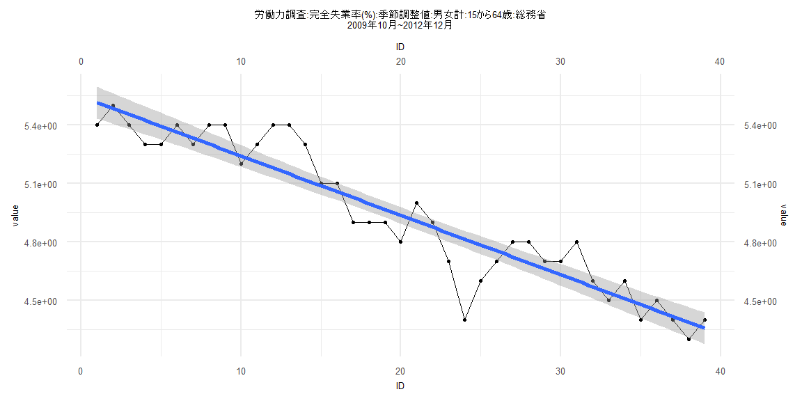
Call:
lm(formula = value ~ ID)

Residuals:
     Min       1Q   Median       3Q      Max
-0.40196 -0.07278 -0.02247  0.07433  0.31214

Coefficients:
              Estimate Std. Error t value            Pr(>|t|)
(Intercept)  4.2852755  0.0277242  154.57 <0.0000000000000002 ***
ID          -0.0243587  0.0005803  -41.98 <0.0000000000000002 ***
---
Signif. codes:  0 '***' 0.001 '**' 0.01 '*' 0.05 '.' 0.1 ' ' 1

Residual standard error: 0.1244 on 80 degrees of freedom
Multiple R-squared:  0.9566,    Adjusted R-squared:  0.956
F-statistic:  1762 on 1 and 80 DF,  p-value: < 0.00000000000000022


    Two-sample Kolmogorov-Smirnov test

data:  lm_residuals and rnorm(n = length(lm_residuals), mean = 0, sd = sd(lm_residuals))
D = 0.18293, p-value = 0.1288
alternative hypothesis: two-sided


    Durbin-Watson test

data:  value ~ ID
DW = 1.1315, p-value = 0.000009666
alternative hypothesis: true autocorrelation is greater than 0


    studentized Breusch-Pagan test

data:  value ~ ID
BP = 0.16569, df = 1, p-value = 0.684


    Box-Ljung test

data:  lm_residuals
X-squared = 12.741, df = 1, p-value = 0.0003577
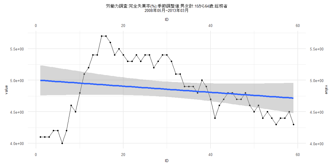
Call:
lm(formula = value ~ ID)

Residuals:
     Min       1Q   Median       3Q      Max
-0.97433 -0.32877  0.01531  0.42292  0.77430

Coefficients:
             Estimate Std. Error t value            Pr(>|t|)
(Intercept)  5.003507   0.122804  40.744 <0.0000000000000002 ***
ID          -0.004863   0.003560  -1.366               0.177
---
Signif. codes:  0 '***' 0.001 '**' 0.01 '*' 0.05 '.' 0.1 ' ' 1

Residual standard error: 0.4657 on 57 degrees of freedom
Multiple R-squared:  0.0317,    Adjusted R-squared:  0.01471
F-statistic: 1.866 on 1 and 57 DF,  p-value: 0.1773


    Two-sample Kolmogorov-Smirnov test

data:  lm_residuals and rnorm(n = length(lm_residuals), mean = 0, sd = sd(lm_residuals))
D = 0.16949, p-value = 0.3674
alternative hypothesis: two-sided


    Durbin-Watson test

data:  value ~ ID
DW = 0.10545, p-value < 0.00000000000000022
alternative hypothesis: true autocorrelation is greater than 0


    studentized Breusch-Pagan test

data:  value ~ ID
BP = 27.165, df = 1, p-value = 0.0000001868


    Box-Ljung test

data:  lm_residuals
X-squared = 51.112, df = 1, p-value = 0.0000000000008722
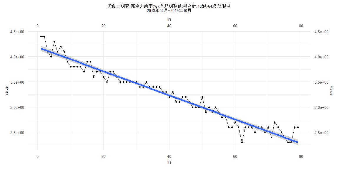
Call:
lm(formula = value ~ ID)

Residuals:
     Min       1Q   Median       3Q      Max
-0.40655 -0.07033 -0.01806  0.06774  0.29921

Coefficients:
              Estimate Std. Error t value            Pr(>|t|)
(Intercept)  4.1863681  0.0274986  152.24 <0.0000000000000002 ***
ID          -0.0238681  0.0005972  -39.97 <0.0000000000000002 ***
---
Signif. codes:  0 '***' 0.001 '**' 0.01 '*' 0.05 '.' 0.1 ' ' 1

Residual standard error: 0.121 on 77 degrees of freedom
Multiple R-squared:  0.954, Adjusted R-squared:  0.9534
F-statistic:  1597 on 1 and 77 DF,  p-value: < 0.00000000000000022


    Two-sample Kolmogorov-Smirnov test

data:  lm_residuals and rnorm(n = length(lm_residuals), mean = 0, sd = sd(lm_residuals))
D = 0.12658, p-value = 0.5543
alternative hypothesis: two-sided


    Durbin-Watson test

data:  value ~ ID
DW = 1.1864, p-value = 0.00004523
alternative hypothesis: true autocorrelation is greater than 0


    studentized Breusch-Pagan test

data:  value ~ ID
BP = 0.44403, df = 1, p-value = 0.5052


    Box-Ljung test

data:  lm_residuals
X-squared = 9.6039, df = 1, p-value = 0.001942