Analysis
[1] "労働力調査:完全失業率(%):季節調整値:男女計:65歳以上:総務省"
     Jan Feb Mar Apr May Jun Jul Aug Sep Oct Nov Dec
1999                                             2.0
2000 2.1 2.5 2.2 2.1 2.2 2.1 2.0 2.2 2.4 2.4 2.3 2.2
2001 2.3 2.5 2.7 2.5 2.8 2.5 2.1 2.2 2.4 2.6 2.1 2.4
2002 2.1 1.7 2.2 2.3 2.2 2.2 2.1 2.1 2.0 2.4 2.4 2.2
2003 2.7 2.5 2.2 2.3 2.3 2.5 2.9 2.6 2.5 2.0 2.5 2.6
2004 2.3 2.3 2.1 2.0 1.6 1.9 2.0 1.8 1.9 2.4 2.3 2.1
2005 1.8 2.1 2.0 1.9 2.5 2.1 1.7 1.7 1.8 1.9 2.0 1.9
2006 2.1 1.9 1.9 1.9 1.9 2.0 2.2 2.4 2.4 2.1 1.7 2.1
2007 2.3 2.3 2.1 2.0 1.8 1.5 1.9 1.9 1.9 1.6 1.7 1.9
2008 1.8 2.0 2.2 2.2 2.5 2.4 2.0 2.2 1.7 2.1 2.5 1.9
2009 1.8 1.9 2.5 2.5 2.3 2.7 2.9 2.5 3.0 2.9 2.6 2.8
2010 2.6 2.3 2.1 2.5 2.5 2.7 2.7 2.6 2.3 2.5 2.4 2.5
2011 2.7 2.7 2.1 2.3 2.0 1.8 2.0 1.9 2.4 2.4 2.0 1.8
2012 2.2 2.3 2.5 2.0 2.7 2.4 2.0 2.0 2.0 1.9 2.2 2.8
2013 2.2 2.2 2.4 2.1 2.0 2.4 2.4 2.5 2.1 2.3 2.6 2.0
2014 2.3 2.0 2.1 2.3 2.1 2.0 2.4 2.4 2.1 2.1 2.0 2.3
2015 2.1 2.1 2.0 2.2 1.9 2.0 1.8 1.9 2.2 1.9 1.8 1.6
2016 1.7 2.0 2.3 1.9 2.1 1.9 1.8 1.9 2.3 2.0 1.9 1.9
2017 2.3 1.8 1.6 1.7 1.9 2.1 1.8 1.6 1.4 1.7 1.8 2.0
2018 1.5 1.7 1.5 1.7 1.7 1.4 1.6 1.7 1.4 1.5 1.4 1.4
2019 1.9 1.5 1.6 1.5 1.1 1.7 2.2 1.7 1.3 1.4
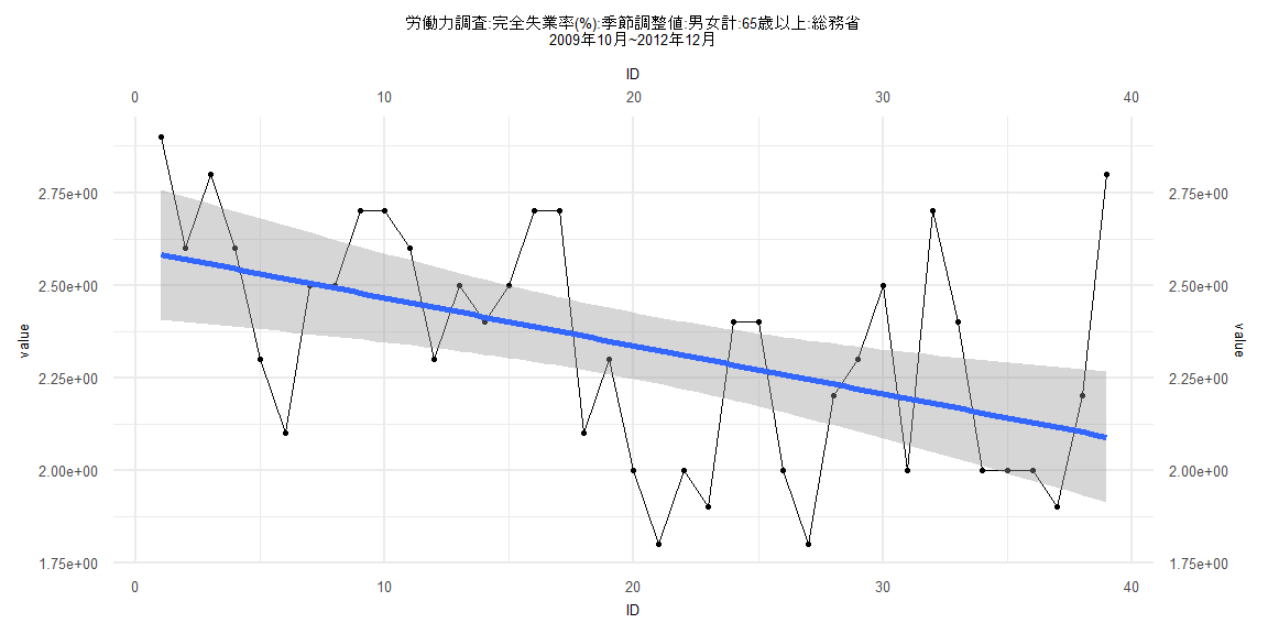
Call:
lm(formula = value ~ ID)

Residuals:
     Min       1Q   Median       3Q      Max
-0.52292 -0.20424  0.00839  0.18435  0.71064

Coefficients:
            Estimate Std. Error t value             Pr(>|t|)
(Intercept)  2.59541    0.09043  28.701 < 0.0000000000000002 ***
ID          -0.01298    0.00394  -3.293              0.00219 **
---
Signif. codes:  0 '***' 0.001 '**' 0.01 '*' 0.05 '.' 0.1 ' ' 1

Residual standard error: 0.277 on 37 degrees of freedom
Multiple R-squared:  0.2266,    Adjusted R-squared:  0.2057
F-statistic: 10.84 on 1 and 37 DF,  p-value: 0.002188


    Two-sample Kolmogorov-Smirnov test

data:  lm_residuals and rnorm(n = length(lm_residuals), mean = 0, sd = sd(lm_residuals))
D = 0.20513, p-value = 0.3888
alternative hypothesis: two-sided


    Durbin-Watson test

data:  value ~ ID
DW = 1.1958, p-value = 0.002365
alternative hypothesis: true autocorrelation is greater than 0


    studentized Breusch-Pagan test

data:  value ~ ID
BP = 2.5033, df = 1, p-value = 0.1136


    Box-Ljung test

data:  lm_residuals
X-squared = 3.6703, df = 1, p-value = 0.05539
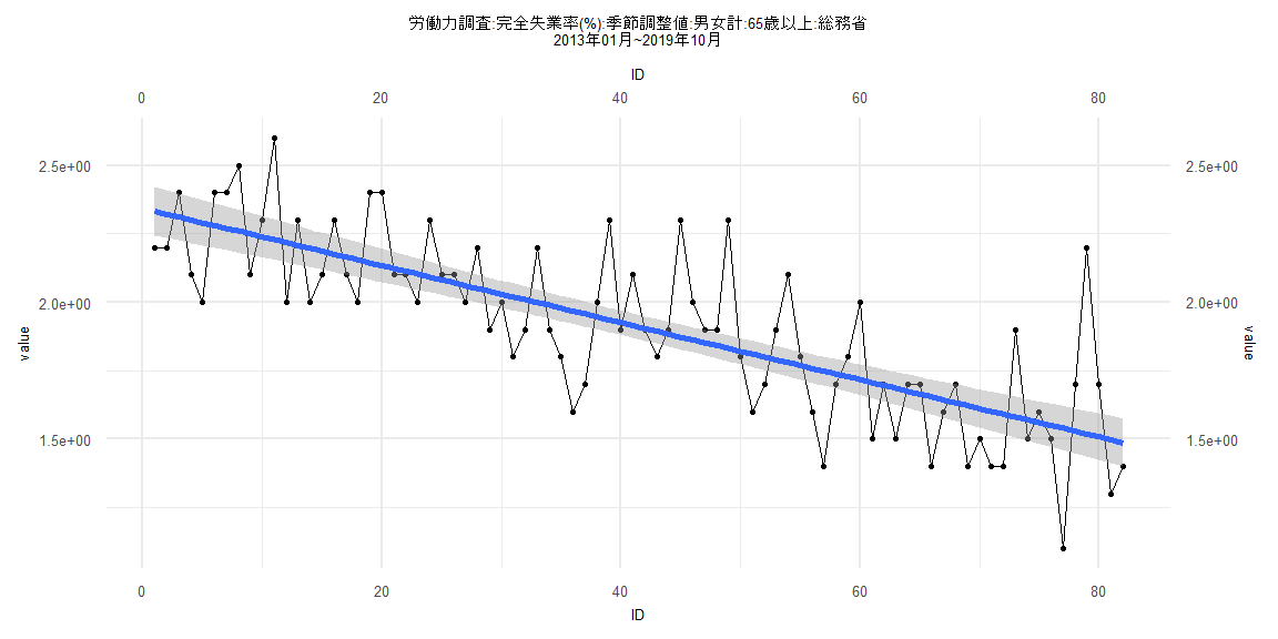
Call:
lm(formula = value ~ ID)

Residuals:
     Min       1Q   Median       3Q      Max
-0.43907 -0.14690 -0.02241  0.11725  0.68181

Coefficients:
              Estimate Std. Error t value            Pr(>|t|)
(Intercept)  2.3430894  0.0454303   51.58 <0.0000000000000002 ***
ID          -0.0104418  0.0009509  -10.98 <0.0000000000000002 ***
---
Signif. codes:  0 '***' 0.001 '**' 0.01 '*' 0.05 '.' 0.1 ' ' 1

Residual standard error: 0.2038 on 80 degrees of freedom
Multiple R-squared:  0.6012,    Adjusted R-squared:  0.5962
F-statistic: 120.6 on 1 and 80 DF,  p-value: < 0.00000000000000022


    Two-sample Kolmogorov-Smirnov test

data:  lm_residuals and rnorm(n = length(lm_residuals), mean = 0, sd = sd(lm_residuals))
D = 0.097561, p-value = 0.8332
alternative hypothesis: two-sided


    Durbin-Watson test

data:  value ~ ID
DW = 1.7609, p-value = 0.1141
alternative hypothesis: true autocorrelation is greater than 0


    studentized Breusch-Pagan test

data:  value ~ ID
BP = 2.4741, df = 1, p-value = 0.1157


    Box-Ljung test

data:  lm_residuals
X-squared = 1.1392, df = 1, p-value = 0.2858
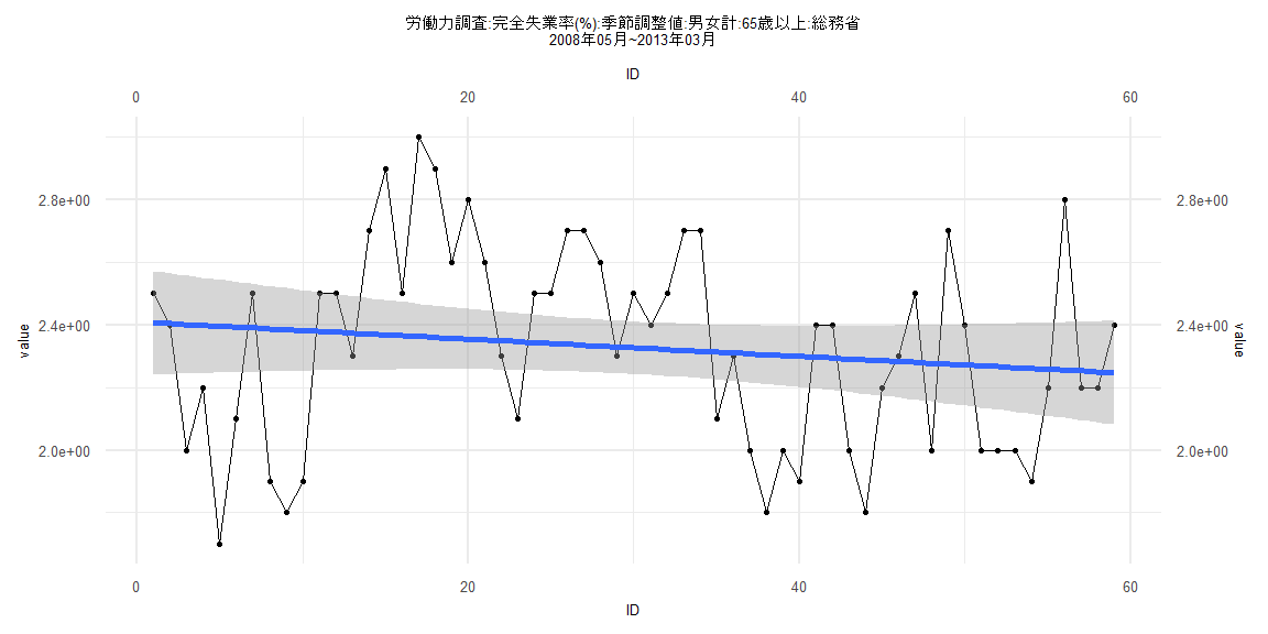
Call:
lm(formula = value ~ ID)

Residuals:
     Min       1Q   Median       3Q      Max
-0.69579 -0.26806  0.01683  0.19898  0.63717

Coefficients:
             Estimate Std. Error t value            Pr(>|t|)
(Intercept)  2.409527   0.084613   28.48 <0.0000000000000002 ***
ID          -0.002747   0.002453   -1.12               0.267
---
Signif. codes:  0 '***' 0.001 '**' 0.01 '*' 0.05 '.' 0.1 ' ' 1

Residual standard error: 0.3208 on 57 degrees of freedom
Multiple R-squared:  0.02153,   Adjusted R-squared:  0.004364
F-statistic: 1.254 on 1 and 57 DF,  p-value: 0.2674


    Two-sample Kolmogorov-Smirnov test

data:  lm_residuals and rnorm(n = length(lm_residuals), mean = 0, sd = sd(lm_residuals))
D = 0.11864, p-value = 0.8052
alternative hypothesis: two-sided


    Durbin-Watson test

data:  value ~ ID
DW = 1.0174, p-value = 0.00001324
alternative hypothesis: true autocorrelation is greater than 0


    studentized Breusch-Pagan test

data:  value ~ ID
BP = 2.7455, df = 1, p-value = 0.09753


    Box-Ljung test

data:  lm_residuals
X-squared = 14.811, df = 1, p-value = 0.0001189
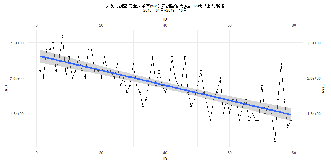
Call:
lm(formula = value ~ ID)

Residuals:
     Min       1Q   Median       3Q      Max
-0.43535 -0.15764 -0.02191  0.11417  0.68588

Coefficients:
             Estimate Std. Error t value             Pr(>|t|)
(Intercept)  2.320740   0.046896   49.49 < 0.0000000000000002 ***
ID          -0.010613   0.001019  -10.42 0.000000000000000229 ***
---
Signif. codes:  0 '***' 0.001 '**' 0.01 '*' 0.05 '.' 0.1 ' ' 1

Residual standard error: 0.2064 on 77 degrees of freedom
Multiple R-squared:  0.5851,    Adjusted R-squared:  0.5797
F-statistic: 108.6 on 1 and 77 DF,  p-value: 0.0000000000000002295


    Two-sample Kolmogorov-Smirnov test

data:  lm_residuals and rnorm(n = length(lm_residuals), mean = 0, sd = sd(lm_residuals))
D = 0.10127, p-value = 0.8161
alternative hypothesis: two-sided


    Durbin-Watson test

data:  value ~ ID
DW = 1.7444, p-value = 0.1034
alternative hypothesis: true autocorrelation is greater than 0


    studentized Breusch-Pagan test

data:  value ~ ID
BP = 1.9236, df = 1, p-value = 0.1655


    Box-Ljung test

data:  lm_residuals
X-squared = 1.1826, df = 1, p-value = 0.2768