Analysis
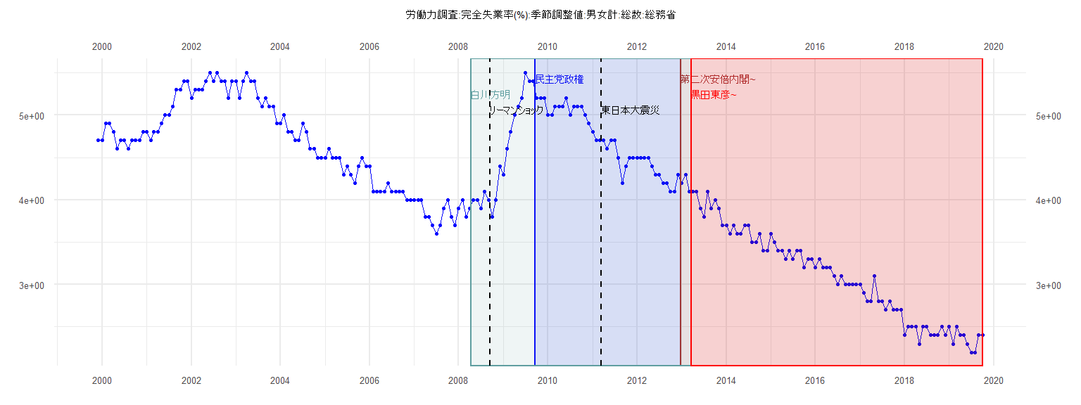
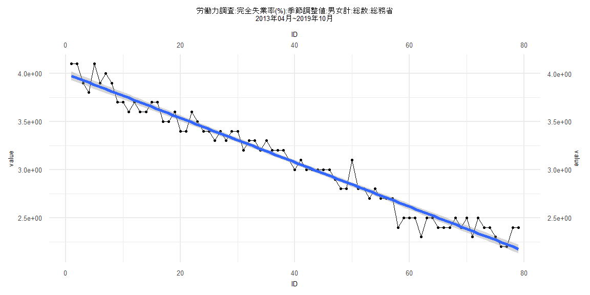
[1] "労働力調査:完全失業率(%):季節調整値:男女計:総数:総務省"
     Jan Feb Mar Apr May Jun Jul Aug Sep Oct Nov Dec
1999                                             4.7
2000 4.7 4.9 4.9 4.8 4.6 4.7 4.7 4.6 4.7 4.7 4.7 4.8
2001 4.8 4.7 4.8 4.8 4.9 5.0 5.0 5.1 5.3 5.3 5.4 5.4
2002 5.2 5.3 5.3 5.3 5.4 5.5 5.4 5.5 5.4 5.4 5.2 5.4
2003 5.4 5.2 5.4 5.5 5.4 5.4 5.2 5.1 5.2 5.1 5.1 4.9
2004 4.9 5.0 4.8 4.8 4.7 4.7 4.9 4.8 4.6 4.6 4.5 4.5
2005 4.5 4.6 4.5 4.5 4.5 4.3 4.4 4.3 4.2 4.4 4.5 4.4
2006 4.4 4.1 4.1 4.1 4.1 4.2 4.1 4.1 4.1 4.1 4.0 4.0
2007 4.0 4.0 4.0 3.8 3.8 3.7 3.6 3.7 3.9 4.0 3.8 3.7
2008 3.9 4.0 3.8 3.9 4.0 4.0 3.9 4.1 4.0 3.8 4.0 4.4
2009 4.3 4.6 4.8 5.0 5.1 5.2 5.5 5.4 5.4 5.2 5.2 5.2
2010 5.0 5.0 5.1 5.1 5.1 5.2 5.0 5.1 5.1 5.1 5.0 4.9
2011 4.8 4.7 4.7 4.7 4.6 4.7 4.7 4.5 4.2 4.4 4.5 4.5
2012 4.5 4.5 4.5 4.5 4.4 4.3 4.3 4.2 4.2 4.1 4.1 4.3
2013 4.2 4.3 4.1 4.1 4.1 3.9 3.8 4.1 3.9 4.0 3.9 3.7
2014 3.7 3.6 3.7 3.6 3.6 3.7 3.7 3.5 3.5 3.6 3.4 3.4
2015 3.6 3.5 3.4 3.4 3.3 3.4 3.3 3.4 3.4 3.2 3.3 3.3
2016 3.2 3.3 3.2 3.2 3.2 3.1 3.0 3.1 3.0 3.0 3.0 3.0
2017 3.0 2.9 2.8 2.8 3.1 2.8 2.8 2.7 2.8 2.7 2.7 2.7
2018 2.4 2.5 2.5 2.5 2.3 2.5 2.5 2.4 2.4 2.4 2.5 2.4
2019 2.5 2.3 2.5 2.4 2.4 2.3 2.2 2.2 2.4 2.4
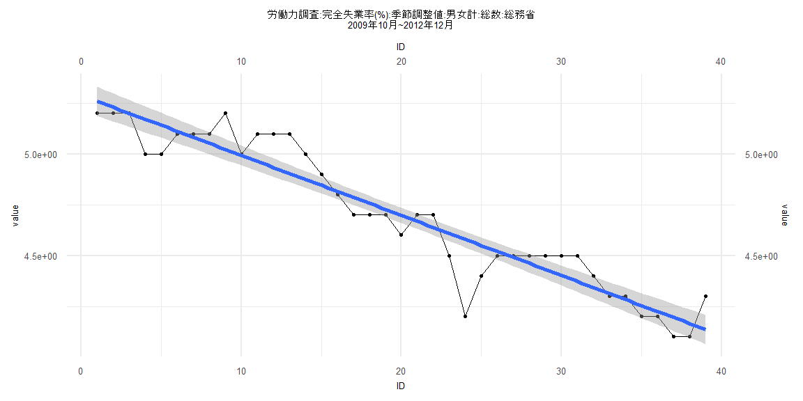
Call:
lm(formula = value ~ ID)

Residuals:
     Min       1Q   Median       3Q      Max
-0.37922 -0.05776  0.00013  0.05945  0.19568

Coefficients:
             Estimate Std. Error t value            Pr(>|t|)
(Intercept)  5.288529   0.036986  142.99 <0.0000000000000002 ***
ID          -0.029555   0.001612  -18.34 <0.0000000000000002 ***
---
Signif. codes:  0 '***' 0.001 '**' 0.01 '*' 0.05 '.' 0.1 ' ' 1

Residual standard error: 0.1133 on 37 degrees of freedom
Multiple R-squared:  0.9009,    Adjusted R-squared:  0.8982
F-statistic: 336.3 on 1 and 37 DF,  p-value: < 0.00000000000000022


    Two-sample Kolmogorov-Smirnov test

data:  lm_residuals and rnorm(n = length(lm_residuals), mean = 0, sd = sd(lm_residuals))
D = 0.12821, p-value = 0.9114
alternative hypothesis: two-sided


    Durbin-Watson test

data:  value ~ ID
DW = 0.86357, p-value = 0.00001877
alternative hypothesis: true autocorrelation is greater than 0


    studentized Breusch-Pagan test

data:  value ~ ID
BP = 0.0046741, df = 1, p-value = 0.9455


    Box-Ljung test

data:  lm_residuals
X-squared = 12.098, df = 1, p-value = 0.0005049
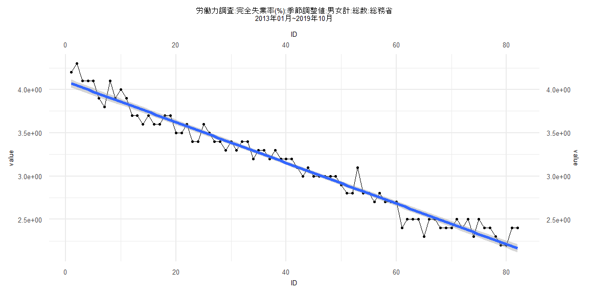
Call:
lm(formula = value ~ ID)

Residuals:
      Min        1Q    Median        3Q       Max
-0.264568 -0.074756 -0.005476  0.059495  0.254248

Coefficients:
              Estimate Std. Error t value            Pr(>|t|)
(Intercept)  4.0927733  0.0234048  174.87 <0.0000000000000002 ***
ID          -0.0235108  0.0004899  -47.99 <0.0000000000000002 ***
---
Signif. codes:  0 '***' 0.001 '**' 0.01 '*' 0.05 '.' 0.1 ' ' 1

Residual standard error: 0.105 on 80 degrees of freedom
Multiple R-squared:  0.9664,    Adjusted R-squared:  0.966
F-statistic:  2303 on 1 and 80 DF,  p-value: < 0.00000000000000022


    Two-sample Kolmogorov-Smirnov test

data:  lm_residuals and rnorm(n = length(lm_residuals), mean = 0, sd = sd(lm_residuals))
D = 0.085366, p-value = 0.9286
alternative hypothesis: two-sided


    Durbin-Watson test

data:  value ~ ID
DW = 1.3606, p-value = 0.0009671
alternative hypothesis: true autocorrelation is greater than 0


    studentized Breusch-Pagan test

data:  value ~ ID
BP = 0.069848, df = 1, p-value = 0.7916


    Box-Ljung test

data:  lm_residuals
X-squared = 6.6029, df = 1, p-value = 0.01018
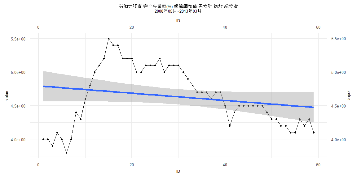
Call:
lm(formula = value ~ ID)

Residuals:
     Min       1Q   Median       3Q      Max
-0.96195 -0.29705 -0.03489  0.37455  0.78670

Coefficients:
             Estimate Std. Error t value            Pr(>|t|)
(Intercept)  4.794389   0.115583  41.480 <0.0000000000000002 ***
ID          -0.005406   0.003351  -1.614               0.112
---
Signif. codes:  0 '***' 0.001 '**' 0.01 '*' 0.05 '.' 0.1 ' ' 1

Residual standard error: 0.4383 on 57 degrees of freedom
Multiple R-squared:  0.04368,   Adjusted R-squared:  0.0269
F-statistic: 2.603 on 1 and 57 DF,  p-value: 0.1122


    Two-sample Kolmogorov-Smirnov test

data:  lm_residuals and rnorm(n = length(lm_residuals), mean = 0, sd = sd(lm_residuals))
D = 0.11864, p-value = 0.8052
alternative hypothesis: two-sided


    Durbin-Watson test

data:  value ~ ID
DW = 0.10346, p-value < 0.00000000000000022
alternative hypothesis: true autocorrelation is greater than 0


    studentized Breusch-Pagan test

data:  value ~ ID
BP = 26.311, df = 1, p-value = 0.0000002906


    Box-Ljung test

data:  lm_residuals
X-squared = 51.77, df = 1, p-value = 0.0000000000006238
Call:
lm(formula = value ~ ID)

Residuals:
      Min        1Q    Median        3Q       Max
-0.268900 -0.075570 -0.007566  0.062527  0.254528

Coefficients:
              Estimate Std. Error t value            Pr(>|t|)
(Intercept)  3.9978578  0.0229041  174.55 <0.0000000000000002 ***
ID          -0.0230477  0.0004974  -46.33 <0.0000000000000002 ***
---
Signif. codes:  0 '***' 0.001 '**' 0.01 '*' 0.05 '.' 0.1 ' ' 1

Residual standard error: 0.1008 on 77 degrees of freedom
Multiple R-squared:  0.9654,    Adjusted R-squared:  0.9649
F-statistic:  2147 on 1 and 77 DF,  p-value: < 0.00000000000000022


    Two-sample Kolmogorov-Smirnov test

data:  lm_residuals and rnorm(n = length(lm_residuals), mean = 0, sd = sd(lm_residuals))
D = 0.17722, p-value = 0.1677
alternative hypothesis: two-sided


    Durbin-Watson test

data:  value ~ ID
DW = 1.4731, p-value = 0.006026
alternative hypothesis: true autocorrelation is greater than 0


    studentized Breusch-Pagan test

data:  value ~ ID
BP = 0.73843, df = 1, p-value = 0.3902


    Box-Ljung test

data:  lm_residuals
X-squared = 4.0314, df = 1, p-value = 0.04466