Analysis
[1] "労働力調査(主要項目):完全失業者(万人):季節調整値:女:総務省"
     Jan Feb Mar Apr May Jun Jul Aug Sep Oct Nov Dec
1999                                             119
2000 122 124 123 128 124 125 120 120 122 121 126 126
2001 128 125 126 124 128 130 130 133 141 133 139 139
2002 136 144 143 136 141 145 141 139 136 137 132 141
2003 145 137 135 140 139 136 135 130 130 130 133 127
2004 126 126 123 125 122 119 121 125 117 118 114 114
2005 114 117 116 117 118 108 119 113 112 119 122 115
2006 111 101 106 106 107 116 109 106 107 105 102 103
2007 107 111 108 102 102  95  93 101 106 107 103 102
2008 104 107 108 110 104 108 108 107 107  99 107 117
2009 118 127 135 130 134 133 138 137 142 135 137 139
2010 132 125 127 130 129 130 126 129 126 128 127 122
2011 120 122 120 115 114 121 119 115 106 109 112 111
2012 118 116 117 115 114 110 112 106 108 109 105 109
2013 106 110 101 107 109  99  93 104 100 106 105 100
2014  98  96  99  95  96  98 103  91  96  95  89  93
2015  94  93  89  90  86  87  91  91  90  81  86  83
2016  85  83  85  86  83  85  81  80  76  79  81  76
2017  80  78  78  78  84  78  74  74  78  77  73  77
2018  68  70  70  66  63  67  69  69  67  65  67  67
2019  75  66  68  71  65  61  64  62  67  70
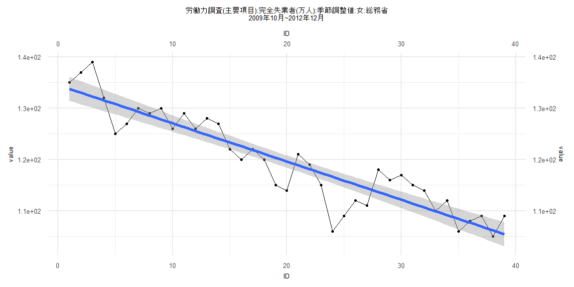
Call:
lm(formula = value ~ ID)

Residuals:
     Min       1Q   Median       3Q      Max
-10.6340  -2.4073   0.4405   2.8660   6.7138

Coefficients:
             Estimate Std. Error t value            Pr(>|t|)
(Intercept) 134.52227    1.21090  111.09 <0.0000000000000002 ***
ID           -0.74534    0.05276  -14.13 <0.0000000000000002 ***
---
Signif. codes:  0 '***' 0.001 '**' 0.01 '*' 0.05 '.' 0.1 ' ' 1

Residual standard error: 3.709 on 37 degrees of freedom
Multiple R-squared:  0.8436,    Adjusted R-squared:  0.8394
F-statistic: 199.5 on 1 and 37 DF,  p-value: < 0.00000000000000022


    Two-sample Kolmogorov-Smirnov test

data:  lm_residuals and rnorm(n = length(lm_residuals), mean = 0, sd = sd(lm_residuals))
D = 0.12821, p-value = 0.9114
alternative hypothesis: two-sided


    Durbin-Watson test

data:  value ~ ID
DW = 1.0343, p-value = 0.0003034
alternative hypothesis: true autocorrelation is greater than 0


    studentized Breusch-Pagan test

data:  value ~ ID
BP = 0.0044327, df = 1, p-value = 0.9469


    Box-Ljung test

data:  lm_residuals
X-squared = 9.2557, df = 1, p-value = 0.002348
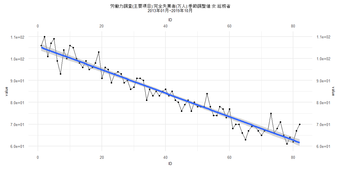
Call:
lm(formula = value ~ ID)

Residuals:
    Min      1Q  Median      3Q     Max
-8.8773 -2.1220 -0.3901  1.8841  8.5359

Coefficients:
            Estimate Std. Error t value            Pr(>|t|)
(Intercept) 105.6332     0.7788  135.63 <0.0000000000000002 ***
ID           -0.5366     0.0163  -32.91 <0.0000000000000002 ***
---
Signif. codes:  0 '***' 0.001 '**' 0.01 '*' 0.05 '.' 0.1 ' ' 1

Residual standard error: 3.494 on 80 degrees of freedom
Multiple R-squared:  0.9312,    Adjusted R-squared:  0.9304
F-statistic:  1083 on 1 and 80 DF,  p-value: < 0.00000000000000022


    Two-sample Kolmogorov-Smirnov test

data:  lm_residuals and rnorm(n = length(lm_residuals), mean = 0, sd = sd(lm_residuals))
D = 0.097561, p-value = 0.8332
alternative hypothesis: two-sided


    Durbin-Watson test

data:  value ~ ID
DW = 1.5999, p-value = 0.02548
alternative hypothesis: true autocorrelation is greater than 0


    studentized Breusch-Pagan test

data:  value ~ ID
BP = 0.022401, df = 1, p-value = 0.881


    Box-Ljung test

data:  lm_residuals
X-squared = 2.2817, df = 1, p-value = 0.1309
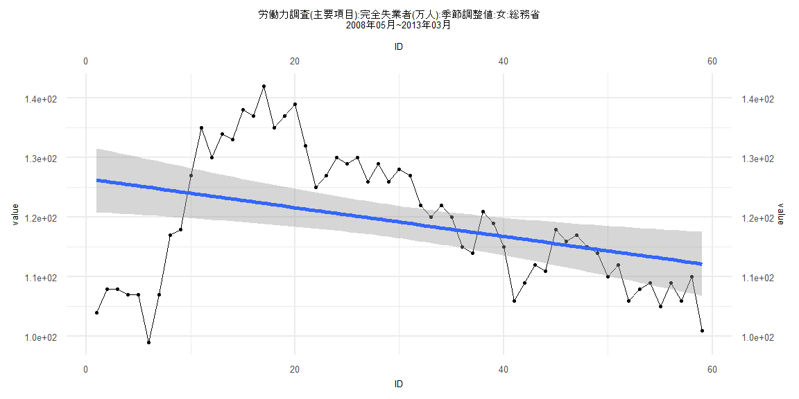
Call:
lm(formula = value ~ ID)

Residuals:
    Min      1Q  Median      3Q     Max
-26.015  -5.961   1.523   8.312  19.649

Coefficients:
             Estimate Std. Error t value             Pr(>|t|)
(Intercept) 126.46756    2.75410  45.920 < 0.0000000000000002 ***
ID           -0.24214    0.07984  -3.033              0.00364 **
---
Signif. codes:  0 '***' 0.001 '**' 0.01 '*' 0.05 '.' 0.1 ' ' 1

Residual standard error: 10.44 on 57 degrees of freedom
Multiple R-squared:  0.139, Adjusted R-squared:  0.1238
F-statistic: 9.199 on 1 and 57 DF,  p-value: 0.003642


    Two-sample Kolmogorov-Smirnov test

data:  lm_residuals and rnorm(n = length(lm_residuals), mean = 0, sd = sd(lm_residuals))
D = 0.10169, p-value = 0.9239
alternative hypothesis: two-sided


    Durbin-Watson test

data:  value ~ ID
DW = 0.19062, p-value < 0.00000000000000022
alternative hypothesis: true autocorrelation is greater than 0


    studentized Breusch-Pagan test

data:  value ~ ID
BP = 24.614, df = 1, p-value = 0.0000007005


    Box-Ljung test

data:  lm_residuals
X-squared = 45.351, df = 1, p-value = 0.00000000001647
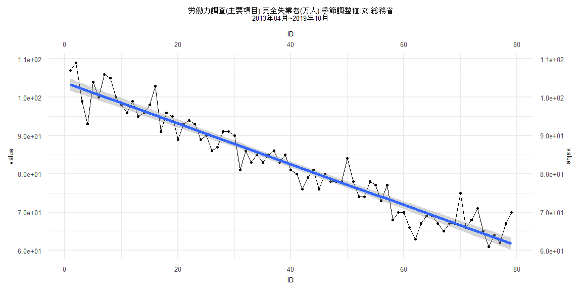
Call:
lm(formula = value ~ ID)

Residuals:
   Min     1Q Median     3Q    Max
-8.713 -2.018 -0.381  1.916  8.476

Coefficients:
             Estimate Std. Error t value            Pr(>|t|)
(Intercept) 103.84518    0.79228  131.07 <0.0000000000000002 ***
ID           -0.53315    0.01721  -30.98 <0.0000000000000002 ***
---
Signif. codes:  0 '***' 0.001 '**' 0.01 '*' 0.05 '.' 0.1 ' ' 1

Residual standard error: 3.488 on 77 degrees of freedom
Multiple R-squared:  0.9258,    Adjusted R-squared:  0.9248
F-statistic:   960 on 1 and 77 DF,  p-value: < 0.00000000000000022


    Two-sample Kolmogorov-Smirnov test

data:  lm_residuals and rnorm(n = length(lm_residuals), mean = 0, sd = sd(lm_residuals))
D = 0.11392, p-value = 0.6878
alternative hypothesis: two-sided


    Durbin-Watson test

data:  value ~ ID
DW = 1.5244, p-value = 0.0116
alternative hypothesis: true autocorrelation is greater than 0


    studentized Breusch-Pagan test

data:  value ~ ID
BP = 0.01876, df = 1, p-value = 0.8911


    Box-Ljung test

data:  lm_residuals
X-squared = 3.087, df = 1, p-value = 0.07892