Analysis
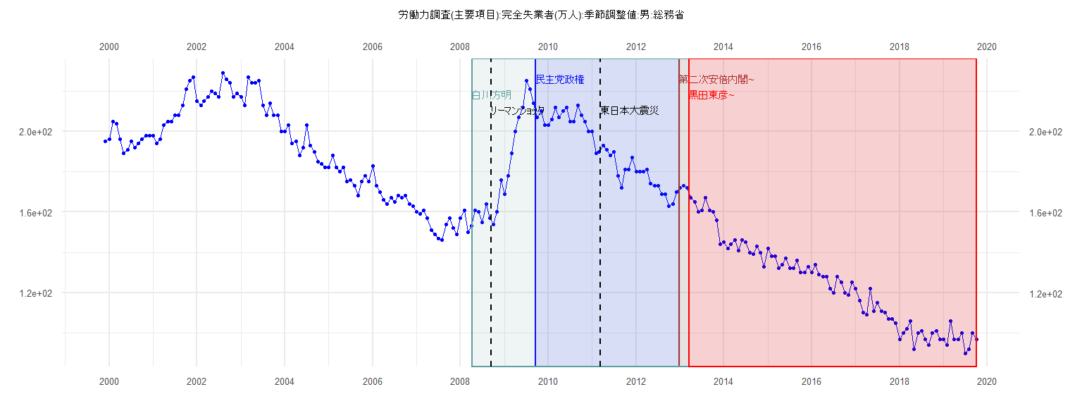
[1] "労働力調査(主要項目):完全失業者(万人):季節調整値:男:総務省"
     Jan Feb Mar Apr May Jun Jul Aug Sep Oct Nov Dec
1999                                             195
2000 196 205 204 196 189 191 195 192 194 196 198 198
2001 198 194 196 203 205 205 208 208 213 221 225 227
2002 215 213 215 217 220 219 217 229 226 224 217 219
2003 217 213 227 224 224 225 213 208 214 208 208 200
2004 200 203 194 195 188 192 203 193 190 185 184 182
2005 182 188 182 180 182 175 176 173 168 175 178 175
2006 183 173 170 166 164 167 165 168 167 168 164 163
2007 160 159 161 157 151 149 147 146 154 157 152 149
2008 157 161 150 153 161 160 155 164 157 154 160 176
2009 169 178 189 200 207 212 225 221 214 207 210 203
2010 203 206 212 207 210 212 205 205 213 208 205 200
2011 200 189 190 193 191 188 190 178 172 181 181 187
2012 180 180 180 181 174 173 173 169 169 163 164 170
2013 172 173 172 167 165 160 161 167 161 160 156 144
2014 145 142 144 146 141 146 145 140 139 143 140 133
2015 142 138 138 132 134 137 132 132 136 130 130 133
2016 130 134 129 128 128 122 120 128 125 120 119 125
2017 122 116 110 109 122 111 115 111 110 107 107 105
2018  97 100 102 106  92 100 101  97  94 100 101  97
2019  97  94 106  97  97 100  90  92 100  97
Call:
lm(formula = value ~ ID)

Residuals:
     Min       1Q   Median       3Q      Max
-13.1692  -3.0346  -0.0077   3.4885  12.4154

Coefficients:
             Estimate Std. Error t value            Pr(>|t|)
(Intercept) 216.00000    1.75435   123.1 <0.0000000000000002 ***
ID           -1.28462    0.07645   -16.8 <0.0000000000000002 ***
---
Signif. codes:  0 '***' 0.001 '**' 0.01 '*' 0.05 '.' 0.1 ' ' 1

Residual standard error: 5.373 on 37 degrees of freedom
Multiple R-squared:  0.8842,    Adjusted R-squared:  0.881
F-statistic: 282.4 on 1 and 37 DF,  p-value: < 0.00000000000000022


    Two-sample Kolmogorov-Smirnov test

data:  lm_residuals and rnorm(n = length(lm_residuals), mean = 0, sd = sd(lm_residuals))
D = 0.12821, p-value = 0.9114
alternative hypothesis: two-sided


    Durbin-Watson test

data:  value ~ ID
DW = 0.8563, p-value = 0.00001639
alternative hypothesis: true autocorrelation is greater than 0


    studentized Breusch-Pagan test

data:  value ~ ID
BP = 2.9456, df = 1, p-value = 0.08611


    Box-Ljung test

data:  lm_residuals
X-squared = 12.094, df = 1, p-value = 0.0005057
Call:
lm(formula = value ~ ID)

Residuals:
     Min       1Q   Median       3Q      Max
-11.5874  -3.1368  -0.8248   2.9476  11.7111

Coefficients:
             Estimate Std. Error t value            Pr(>|t|)
(Intercept) 164.02800    1.18542  138.37 <0.0000000000000002 ***
ID           -0.92985    0.02481  -37.48 <0.0000000000000002 ***
---
Signif. codes:  0 '***' 0.001 '**' 0.01 '*' 0.05 '.' 0.1 ' ' 1

Residual standard error: 5.318 on 80 degrees of freedom
Multiple R-squared:  0.9461,    Adjusted R-squared:  0.9454
F-statistic:  1404 on 1 and 80 DF,  p-value: < 0.00000000000000022


    Two-sample Kolmogorov-Smirnov test

data:  lm_residuals and rnorm(n = length(lm_residuals), mean = 0, sd = sd(lm_residuals))
D = 0.10976, p-value = 0.7099
alternative hypothesis: two-sided


    Durbin-Watson test

data:  value ~ ID
DW = 0.93587, p-value = 0.00000004088
alternative hypothesis: true autocorrelation is greater than 0


    studentized Breusch-Pagan test

data:  value ~ ID
BP = 0.52856, df = 1, p-value = 0.4672


    Box-Ljung test

data:  lm_residuals
X-squared = 20.901, df = 1, p-value = 0.000004837
Call:
lm(formula = value ~ ID)

Residuals:
    Min      1Q  Median      3Q     Max
-37.553 -12.583  -1.632  17.352  35.104

Coefficients:
            Estimate Std. Error t value            Pr(>|t|)
(Intercept) 192.6569     4.9942  38.576 <0.0000000000000002 ***
ID           -0.1840     0.1448  -1.271               0.209
---
Signif. codes:  0 '***' 0.001 '**' 0.01 '*' 0.05 '.' 0.1 ' ' 1

Residual standard error: 18.94 on 57 degrees of freedom
Multiple R-squared:  0.02757,   Adjusted R-squared:  0.01051
F-statistic: 1.616 on 1 and 57 DF,  p-value: 0.2088


    Two-sample Kolmogorov-Smirnov test

data:  lm_residuals and rnorm(n = length(lm_residuals), mean = 0, sd = sd(lm_residuals))
D = 0.16949, p-value = 0.3674
alternative hypothesis: two-sided


    Durbin-Watson test

data:  value ~ ID
DW = 0.10493, p-value < 0.00000000000000022
alternative hypothesis: true autocorrelation is greater than 0


    studentized Breusch-Pagan test

data:  value ~ ID
BP = 26.409, df = 1, p-value = 0.0000002763


    Box-Ljung test

data:  lm_residuals
X-squared = 52.63, df = 1, p-value = 0.0000000000004028
Call:
lm(formula = value ~ ID)

Residuals:
     Min       1Q   Median       3Q      Max
-11.8700  -3.0684  -0.8539   3.0536  11.8605

Coefficients:
             Estimate Std. Error t value            Pr(>|t|)
(Intercept) 159.63681    1.12862   141.4 <0.0000000000000002 ***
ID           -0.89946    0.02451   -36.7 <0.0000000000000002 ***
---
Signif. codes:  0 '***' 0.001 '**' 0.01 '*' 0.05 '.' 0.1 ' ' 1

Residual standard error: 4.968 on 77 degrees of freedom
Multiple R-squared:  0.9459,    Adjusted R-squared:  0.9452
F-statistic:  1347 on 1 and 77 DF,  p-value: < 0.00000000000000022


    Two-sample Kolmogorov-Smirnov test

data:  lm_residuals and rnorm(n = length(lm_residuals), mean = 0, sd = sd(lm_residuals))
D = 0.088608, p-value = 0.9184
alternative hypothesis: two-sided


    Durbin-Watson test

data:  value ~ ID
DW = 1.1035, p-value = 0.00000692
alternative hypothesis: true autocorrelation is greater than 0


    studentized Breusch-Pagan test

data:  value ~ ID
BP = 0.016694, df = 1, p-value = 0.8972


    Box-Ljung test

data:  lm_residuals
X-squared = 13.902, df = 1, p-value = 0.0001926