Analysis
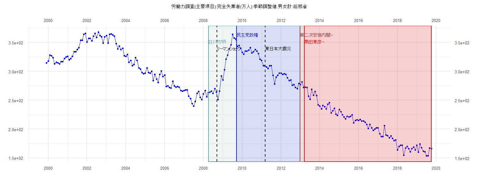
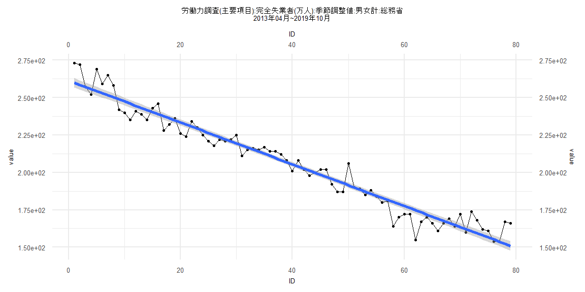
[1] "労働力調査(主要項目):完全失業者(万人):季節調整値:男女計:総務省"
     Jan Feb Mar Apr May Jun Jul Aug Sep Oct Nov Dec
1999                                             315
2000 318 328 327 324 313 316 315 313 317 317 322 325
2001 326 320 322 326 334 334 338 341 354 354 364 366
2002 351 357 357 353 361 366 359 368 362 360 349 360
2003 362 349 364 365 363 361 348 339 344 338 340 327
2004 326 329 316 319 310 312 324 319 306 304 298 296
2005 297 306 298 297 300 284 295 287 281 295 301 291
2006 294 274 275 272 271 283 275 273 274 273 267 266
2007 267 268 268 257 253 244 240 248 262 265 255 251
2008 261 267 256 263 264 266 262 270 264 251 266 292
2009 285 303 321 328 339 346 364 358 356 343 345 340
2010 333 330 335 335 337 341 332 334 338 335 331 321
2011 319 310 310 308 305 310 310 293 278 290 293 297
2012 297 295 296 295 289 284 285 276 277 272 270 279
2013 277 282 272 273 272 257 252 269 259 265 258 242
2014 240 235 241 239 235 243 246 228 232 236 226 224
2015 234 230 225 221 218 222 221 222 225 211 215 216
2016 215 217 214 214 212 208 201 208 202 198 200 202
2017 202 192 187 187 206 190 189 185 188 184 180 181
2018 164 170 172 172 155 167 170 166 161 166 169 164
2019 172 160 174 168 162 161 154 154 167 166
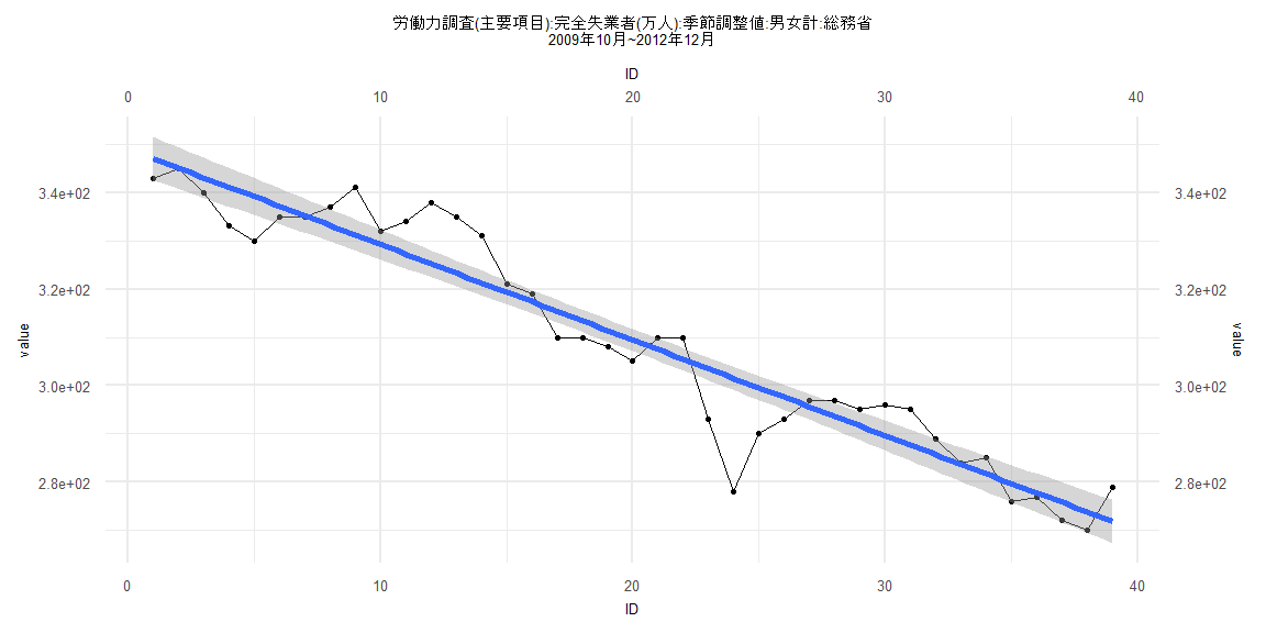
Call:
lm(formula = value ~ ID)

Residuals:
     Min       1Q   Median       3Q      Max
-23.5217  -3.8114   0.2852   3.6070  12.7358

Coefficients:
            Estimate Std. Error t value            Pr(>|t|)
(Intercept) 349.0067     2.3096  151.11 <0.0000000000000002 ***
ID           -1.9785     0.1006  -19.66 <0.0000000000000002 ***
---
Signif. codes:  0 '***' 0.001 '**' 0.01 '*' 0.05 '.' 0.1 ' ' 1

Residual standard error: 7.074 on 37 degrees of freedom
Multiple R-squared:  0.9126,    Adjusted R-squared:  0.9103
F-statistic: 386.5 on 1 and 37 DF,  p-value: < 0.00000000000000022


    Two-sample Kolmogorov-Smirnov test

data:  lm_residuals and rnorm(n = length(lm_residuals), mean = 0, sd = sd(lm_residuals))
D = 0.25641, p-value = 0.1547
alternative hypothesis: two-sided


    Durbin-Watson test

data:  value ~ ID
DW = 0.71274, p-value = 0.0000007817
alternative hypothesis: true autocorrelation is greater than 0


    studentized Breusch-Pagan test

data:  value ~ ID
BP = 0.032332, df = 1, p-value = 0.8573


    Box-Ljung test

data:  lm_residuals
X-squared = 16.459, df = 1, p-value = 0.00004971
Call:
lm(formula = value ~ ID)

Residuals:
     Min       1Q   Median       3Q      Max
-19.3346  -5.1624  -0.2806   3.9110  17.3154

Coefficients:
             Estimate Std. Error t value            Pr(>|t|)
(Intercept) 267.55285    1.65384  161.78 <0.0000000000000002 ***
ID           -1.43413    0.03462  -41.43 <0.0000000000000002 ***
---
Signif. codes:  0 '***' 0.001 '**' 0.01 '*' 0.05 '.' 0.1 ' ' 1

Residual standard error: 7.42 on 80 degrees of freedom
Multiple R-squared:  0.9555,    Adjusted R-squared:  0.9549
F-statistic:  1716 on 1 and 80 DF,  p-value: < 0.00000000000000022


    Two-sample Kolmogorov-Smirnov test

data:  lm_residuals and rnorm(n = length(lm_residuals), mean = 0, sd = sd(lm_residuals))
D = 0.15854, p-value = 0.2552
alternative hypothesis: two-sided


    Durbin-Watson test

data:  value ~ ID
DW = 1.0307, p-value = 0.0000007116
alternative hypothesis: true autocorrelation is greater than 0


    studentized Breusch-Pagan test

data:  value ~ ID
BP = 0.098584, df = 1, p-value = 0.7535


    Box-Ljung test

data:  lm_residuals
X-squared = 16.613, df = 1, p-value = 0.00004584
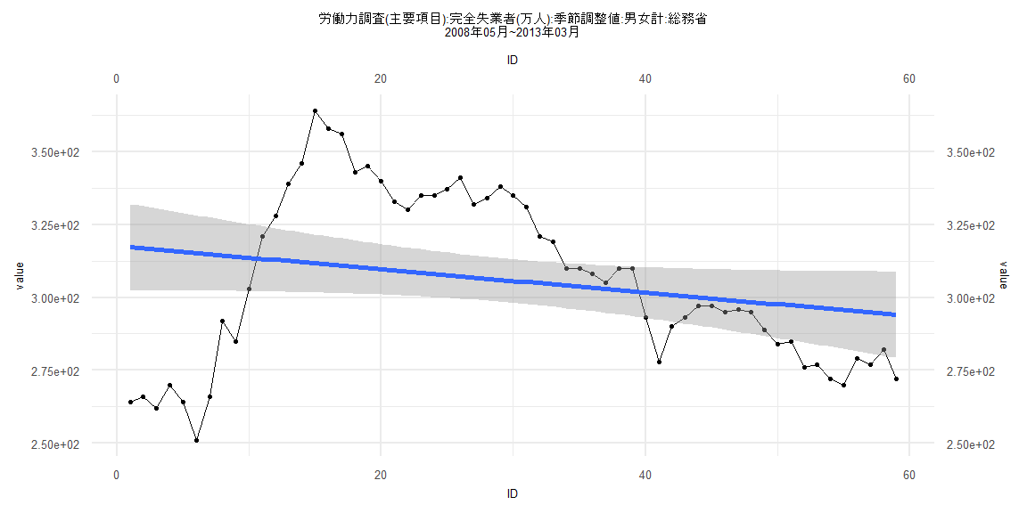
Call:
lm(formula = value ~ ID)

Residuals:
    Min      1Q  Median      3Q     Max
-64.264 -18.658  -2.659  26.138  52.337

Coefficients:
            Estimate Std. Error t value            Pr(>|t|)
(Intercept) 317.6645     7.5788  41.915 <0.0000000000000002 ***
ID           -0.4001     0.2197  -1.821              0.0738 .
---
Signif. codes:  0 '***' 0.001 '**' 0.01 '*' 0.05 '.' 0.1 ' ' 1

Residual standard error: 28.74 on 57 degrees of freedom
Multiple R-squared:  0.05499,   Adjusted R-squared:  0.03841
F-statistic: 3.317 on 1 and 57 DF,  p-value: 0.07383


    Two-sample Kolmogorov-Smirnov test

data:  lm_residuals and rnorm(n = length(lm_residuals), mean = 0, sd = sd(lm_residuals))
D = 0.13559, p-value = 0.6544
alternative hypothesis: two-sided


    Durbin-Watson test

data:  value ~ ID
DW = 0.089384, p-value < 0.00000000000000022
alternative hypothesis: true autocorrelation is greater than 0


    studentized Breusch-Pagan test

data:  value ~ ID
BP = 27.047, df = 1, p-value = 0.0000001986


    Box-Ljung test

data:  lm_residuals
X-squared = 52.521, df = 1, p-value = 0.0000000000004257
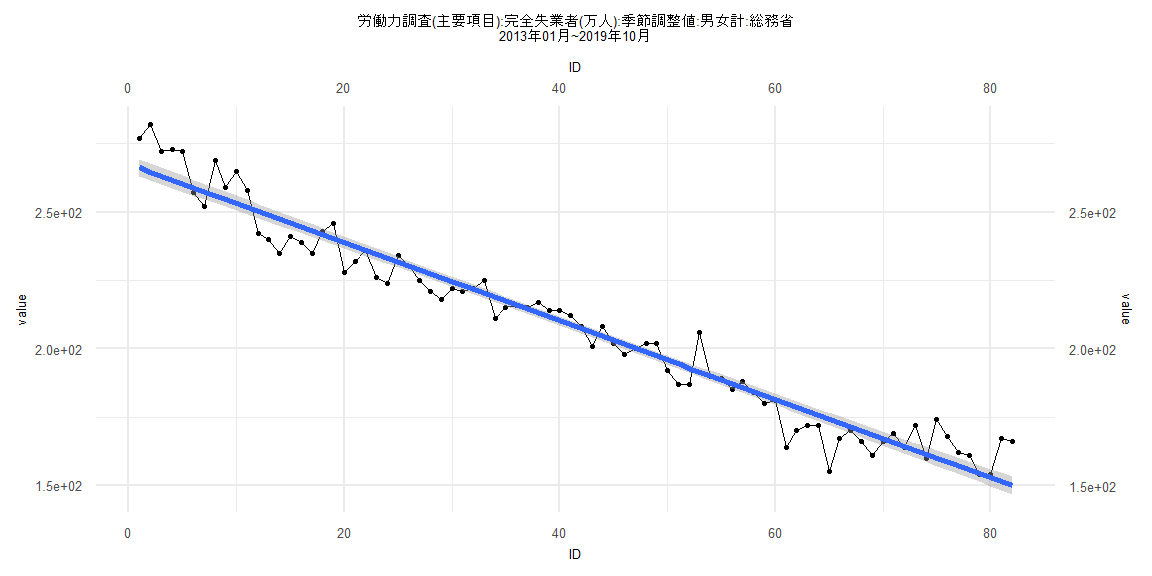
Call:
lm(formula = value ~ ID)

Residuals:
     Min       1Q   Median       3Q      Max
-19.6793  -4.2869  -0.6233   3.8837  15.0731

Coefficients:
             Estimate Std. Error t value            Pr(>|t|)
(Intercept) 261.30574    1.60344  162.97 <0.0000000000000002 ***
ID           -1.39720    0.03482  -40.12 <0.0000000000000002 ***
---
Signif. codes:  0 '***' 0.001 '**' 0.01 '*' 0.05 '.' 0.1 ' ' 1

Residual standard error: 7.058 on 77 degrees of freedom
Multiple R-squared:  0.9543,    Adjusted R-squared:  0.9538
F-statistic:  1610 on 1 and 77 DF,  p-value: < 0.00000000000000022


    Two-sample Kolmogorov-Smirnov test

data:  lm_residuals and rnorm(n = length(lm_residuals), mean = 0, sd = sd(lm_residuals))
D = 0.10127, p-value = 0.8161
alternative hypothesis: two-sided


    Durbin-Watson test

data:  value ~ ID
DW = 1.1518, p-value = 0.00002127
alternative hypothesis: true autocorrelation is greater than 0


    studentized Breusch-Pagan test

data:  value ~ ID
BP = 0.053319, df = 1, p-value = 0.8174


    Box-Ljung test

data:  lm_residuals
X-squared = 11.363, df = 1, p-value = 0.0007492