Analysis
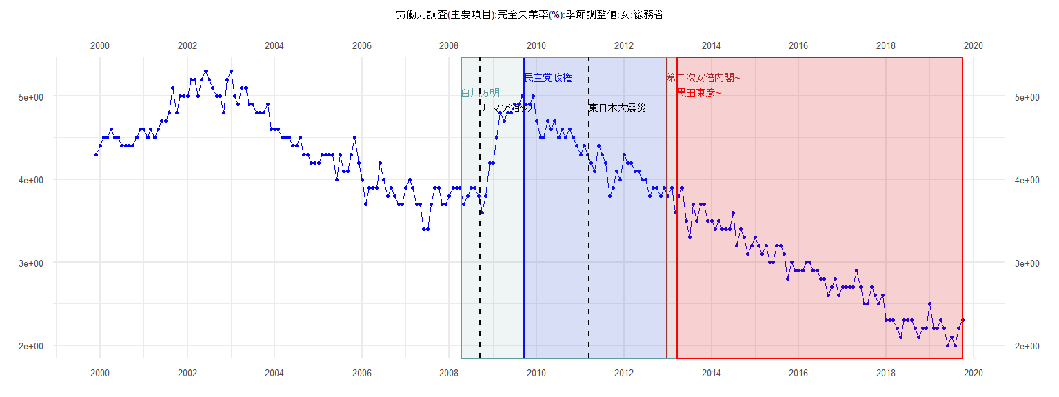
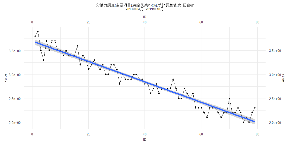
[1] "労働力調査(主要項目):完全失業率(%):季節調整値:女:総務省"
     Jan Feb Mar Apr May Jun Jul Aug Sep Oct Nov Dec
1999                                             4.3
2000 4.4 4.5 4.5 4.6 4.5 4.5 4.4 4.4 4.4 4.4 4.5 4.6
2001 4.6 4.5 4.6 4.5 4.6 4.7 4.7 4.8 5.1 4.8 5.0 5.0
2002 5.0 5.2 5.2 5.0 5.2 5.3 5.2 5.1 5.0 5.0 4.8 5.2
2003 5.3 5.0 4.9 5.1 5.1 4.9 4.9 4.8 4.8 4.8 4.9 4.6
2004 4.6 4.6 4.5 4.5 4.5 4.4 4.4 4.5 4.3 4.3 4.2 4.2
2005 4.2 4.3 4.3 4.3 4.3 4.0 4.3 4.1 4.1 4.3 4.5 4.2
2006 4.0 3.7 3.9 3.9 3.9 4.2 4.0 3.8 3.9 3.8 3.7 3.7
2007 3.9 4.0 3.9 3.7 3.7 3.4 3.4 3.7 3.9 3.9 3.7 3.7
2008 3.8 3.9 3.9 3.9 3.7 3.8 3.9 3.9 3.8 3.6 3.8 4.2
2009 4.2 4.5 4.8 4.7 4.8 4.8 4.9 4.9 5.0 4.9 4.9 5.0
2010 4.7 4.5 4.5 4.7 4.6 4.7 4.5 4.6 4.5 4.6 4.5 4.4
2011 4.3 4.4 4.3 4.2 4.1 4.4 4.3 4.2 3.8 3.9 4.1 4.0
2012 4.3 4.2 4.2 4.1 4.1 4.0 4.0 3.8 3.9 3.9 3.8 3.9
2013 3.8 3.9 3.6 3.8 3.9 3.5 3.3 3.7 3.5 3.7 3.7 3.5
2014 3.5 3.4 3.5 3.4 3.4 3.4 3.6 3.2 3.4 3.3 3.1 3.2
2015 3.3 3.2 3.1 3.2 3.0 3.0 3.2 3.2 3.1 2.8 3.0 2.9
2016 2.9 2.9 3.0 3.0 2.9 2.9 2.8 2.8 2.6 2.7 2.8 2.6
2017 2.7 2.7 2.7 2.7 2.9 2.7 2.5 2.5 2.7 2.6 2.5 2.6
2018 2.3 2.3 2.3 2.2 2.1 2.3 2.3 2.3 2.2 2.1 2.2 2.2
2019 2.5 2.2 2.2 2.3 2.2 2.0 2.1 2.0 2.2 2.3
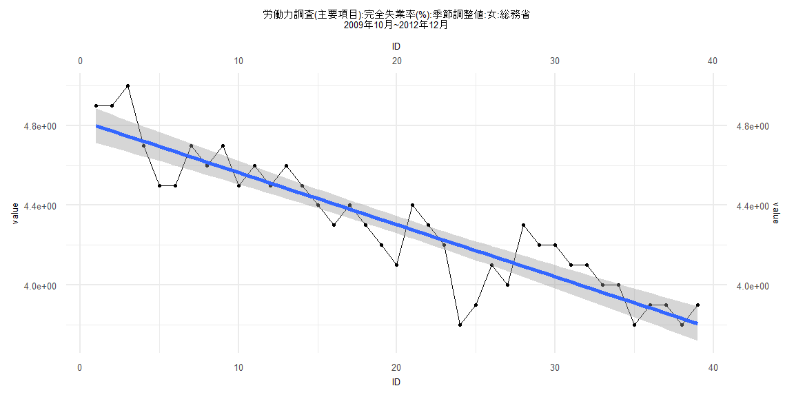
Call:
lm(formula = value ~ ID)

Residuals:
     Min       1Q   Median       3Q      Max
-0.39795 -0.05949  0.01897  0.09744  0.25282

Coefficients:
             Estimate Std. Error t value             Pr(>|t|)
(Intercept)  4.825641   0.043960  109.77 < 0.0000000000000002 ***
ID          -0.026154   0.001916  -13.65 0.000000000000000507 ***
---
Signif. codes:  0 '***' 0.001 '**' 0.01 '*' 0.05 '.' 0.1 ' ' 1

Residual standard error: 0.1346 on 37 degrees of freedom
Multiple R-squared:  0.8344,    Adjusted R-squared:  0.8299
F-statistic: 186.4 on 1 and 37 DF,  p-value: 0.000000000000000507


    Two-sample Kolmogorov-Smirnov test

data:  lm_residuals and rnorm(n = length(lm_residuals), mean = 0, sd = sd(lm_residuals))
D = 0.15385, p-value = 0.7523
alternative hypothesis: two-sided


    Durbin-Watson test

data:  value ~ ID
DW = 1.2431, p-value = 0.00396
alternative hypothesis: true autocorrelation is greater than 0


    studentized Breusch-Pagan test

data:  value ~ ID
BP = 0.035284, df = 1, p-value = 0.851


    Box-Ljung test

data:  lm_residuals
X-squared = 5.5843, df = 1, p-value = 0.01812
Call:
lm(formula = value ~ ID)

Residuals:
      Min        1Q    Median        3Q       Max
-0.315091 -0.084415 -0.004176  0.076243  0.299569

Coefficients:
              Estimate Std. Error t value            Pr(>|t|)
(Intercept)  3.7651310  0.0280281  134.33 <0.0000000000000002 ***
ID          -0.0214342  0.0005867  -36.54 <0.0000000000000002 ***
---
Signif. codes:  0 '***' 0.001 '**' 0.01 '*' 0.05 '.' 0.1 ' ' 1

Residual standard error: 0.1257 on 80 degrees of freedom
Multiple R-squared:  0.9435,    Adjusted R-squared:  0.9428
F-statistic:  1335 on 1 and 80 DF,  p-value: < 0.00000000000000022


    Two-sample Kolmogorov-Smirnov test

data:  lm_residuals and rnorm(n = length(lm_residuals), mean = 0, sd = sd(lm_residuals))
D = 0.14634, p-value = 0.3453
alternative hypothesis: two-sided


    Durbin-Watson test

data:  value ~ ID
DW = 1.5992, p-value = 0.0253
alternative hypothesis: true autocorrelation is greater than 0


    studentized Breusch-Pagan test

data:  value ~ ID
BP = 0.089768, df = 1, p-value = 0.7645


    Box-Ljung test

data:  lm_residuals
X-squared = 2.3239, df = 1, p-value = 0.1274
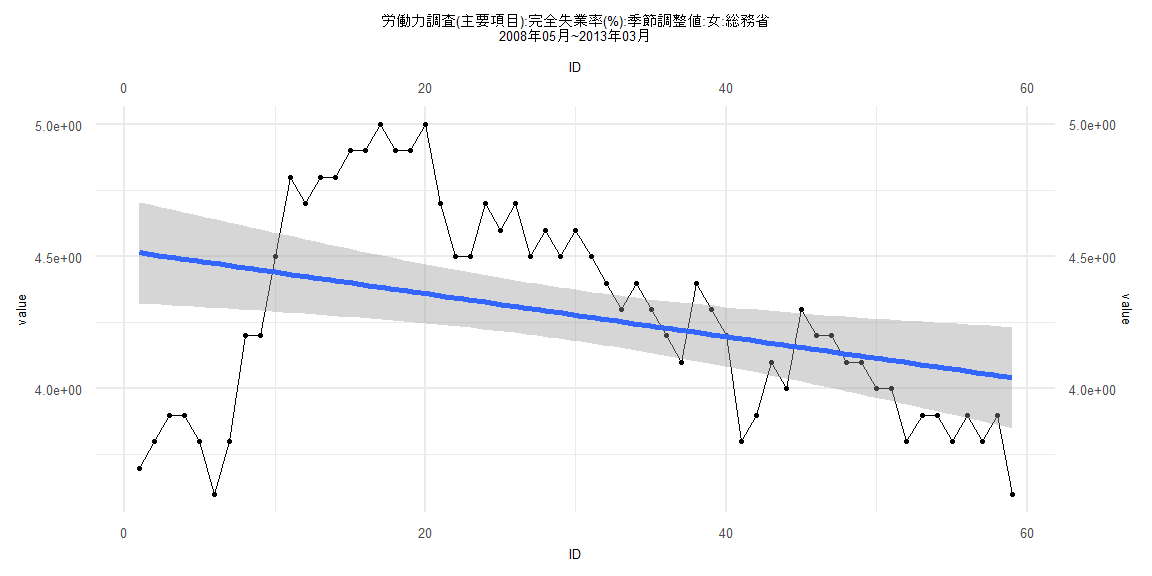
Call:
lm(formula = value ~ ID)

Residuals:
     Min       1Q   Median       3Q      Max
-0.87364 -0.21981  0.05248  0.27827  0.64050

Coefficients:
             Estimate Std. Error t value             Pr(>|t|)
(Intercept)  4.522560   0.098081  46.111 < 0.0000000000000002 ***
ID          -0.008153   0.002843  -2.868              0.00579 **
---
Signif. codes:  0 '***' 0.001 '**' 0.01 '*' 0.05 '.' 0.1 ' ' 1

Residual standard error: 0.3719 on 57 degrees of freedom
Multiple R-squared:  0.1261,    Adjusted R-squared:  0.1107
F-statistic: 8.223 on 1 and 57 DF,  p-value: 0.005789


    Two-sample Kolmogorov-Smirnov test

data:  lm_residuals and rnorm(n = length(lm_residuals), mean = 0, sd = sd(lm_residuals))
D = 0.10169, p-value = 0.9239
alternative hypothesis: two-sided


    Durbin-Watson test

data:  value ~ ID
DW = 0.18674, p-value < 0.00000000000000022
alternative hypothesis: true autocorrelation is greater than 0


    studentized Breusch-Pagan test

data:  value ~ ID
BP = 24.587, df = 1, p-value = 0.0000007103


    Box-Ljung test

data:  lm_residuals
X-squared = 45.065, df = 1, p-value = 0.00000000001906
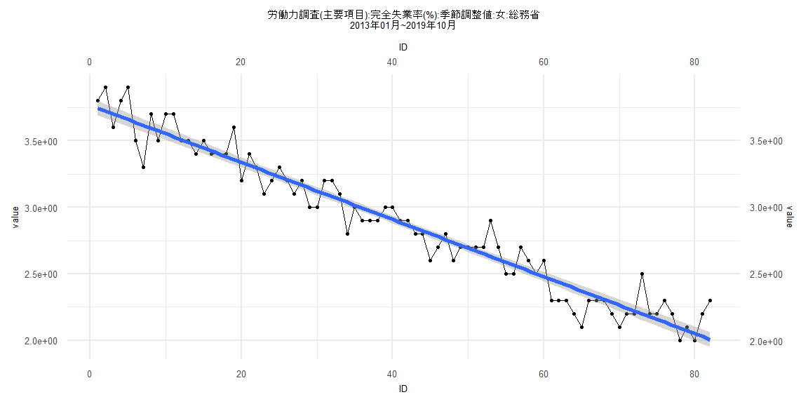
Call:
lm(formula = value ~ ID)

Residuals:
      Min        1Q    Median        3Q       Max
-0.308481 -0.080206 -0.001994  0.076282  0.297152

Coefficients:
              Estimate Std. Error t value            Pr(>|t|)
(Intercept)  3.6936709  0.0285831  129.23 <0.0000000000000002 ***
ID          -0.0212975  0.0006208  -34.31 <0.0000000000000002 ***
---
Signif. codes:  0 '***' 0.001 '**' 0.01 '*' 0.05 '.' 0.1 ' ' 1

Residual standard error: 0.1258 on 77 degrees of freedom
Multiple R-squared:  0.9386,    Adjusted R-squared:  0.9378
F-statistic:  1177 on 1 and 77 DF,  p-value: < 0.00000000000000022


    Two-sample Kolmogorov-Smirnov test

data:  lm_residuals and rnorm(n = length(lm_residuals), mean = 0, sd = sd(lm_residuals))
D = 0.050633, p-value = 1
alternative hypothesis: two-sided


    Durbin-Watson test

data:  value ~ ID
DW = 1.5435, p-value = 0.01457
alternative hypothesis: true autocorrelation is greater than 0


    studentized Breusch-Pagan test

data:  value ~ ID
BP = 0.060691, df = 1, p-value = 0.8054


    Box-Ljung test

data:  lm_residuals
X-squared = 2.88, df = 1, p-value = 0.08968