Analysis
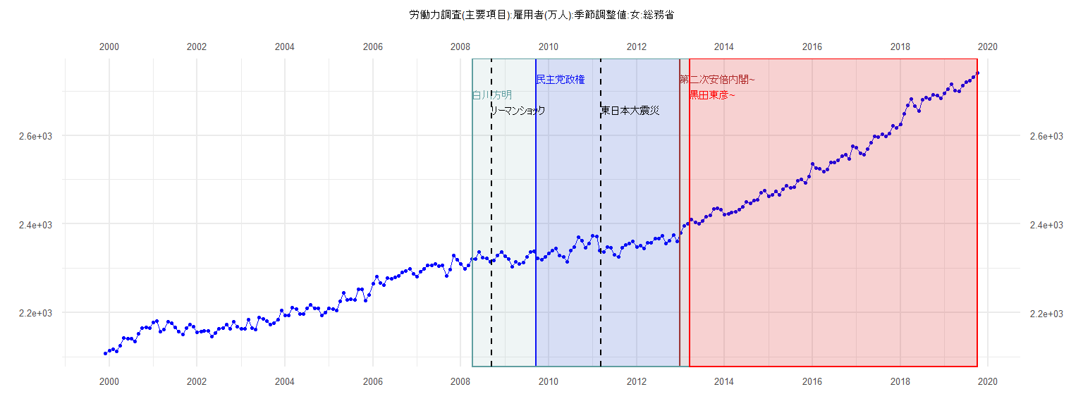
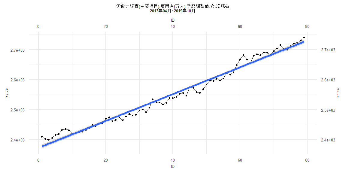
[1] "労働力調査(主要項目):雇用者(万人):季節調整値:女:総務省"
      Jan  Feb  Mar  Apr  May  Jun  Jul  Aug  Sep  Oct  Nov  Dec
1999                                                        2108
2000 2114 2117 2112 2125 2142 2140 2140 2135 2152 2165 2166 2165
2001 2177 2181 2156 2161 2179 2175 2167 2157 2151 2164 2172 2168
2002 2155 2157 2158 2159 2145 2153 2163 2164 2173 2163 2179 2168
2003 2163 2163 2184 2165 2161 2188 2186 2180 2173 2176 2183 2205
2004 2193 2194 2211 2208 2197 2197 2210 2217 2210 2210 2194 2199
2005 2210 2208 2205 2225 2245 2228 2230 2229 2253 2253 2227 2239
2006 2265 2281 2267 2261 2277 2276 2279 2282 2290 2293 2298 2287
2007 2281 2292 2298 2306 2306 2309 2304 2306 2282 2297 2329 2319
2008 2310 2299 2307 2321 2321 2336 2324 2322 2314 2317 2329 2336
2009 2327 2321 2303 2315 2310 2313 2325 2337 2338 2323 2319 2325
2010 2333 2340 2345 2328 2326 2314 2339 2347 2370 2362 2346 2355
2011 2374 2372 2340 2336 2347 2346 2330 2326 2346 2352 2356 2360
2012 2347 2351 2344 2357 2358 2367 2367 2373 2355 2362 2375 2360
2013 2379 2396 2401 2410 2403 2400 2406 2416 2419 2433 2436 2432
2014 2421 2423 2425 2427 2432 2439 2449 2446 2453 2454 2470 2475
2015 2462 2466 2474 2465 2478 2486 2481 2483 2498 2501 2492 2507
2016 2535 2526 2524 2518 2523 2539 2539 2543 2553 2556 2547 2575
2017 2573 2559 2556 2569 2584 2597 2596 2603 2598 2604 2622 2617
2018 2625 2649 2668 2682 2667 2655 2680 2685 2682 2691 2690 2684
2019 2695 2704 2716 2702 2700 2713 2720 2723 2731 2741
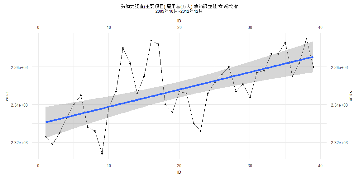
Call:
lm(formula = value ~ ID)

Residuals:
    Min      1Q  Median      3Q     Max
-24.778  -7.649  -1.034   6.589  29.644

Coefficients:
             Estimate Std. Error t value             Pr(>|t|)
(Intercept) 2329.6775     4.2141 552.823 < 0.0000000000000002 ***
ID             0.9174     0.1836   4.996            0.0000143 ***
---
Signif. codes:  0 '***' 0.001 '**' 0.01 '*' 0.05 '.' 0.1 ' ' 1

Residual standard error: 12.91 on 37 degrees of freedom
Multiple R-squared:  0.4028,    Adjusted R-squared:  0.3867
F-statistic: 24.96 on 1 and 37 DF,  p-value: 0.00001428


    Two-sample Kolmogorov-Smirnov test

data:  lm_residuals and rnorm(n = length(lm_residuals), mean = 0, sd = sd(lm_residuals))
D = 0.17949, p-value = 0.5622
alternative hypothesis: two-sided


    Durbin-Watson test

data:  value ~ ID
DW = 0.93539, p-value = 0.00006615
alternative hypothesis: true autocorrelation is greater than 0


    studentized Breusch-Pagan test

data:  value ~ ID
BP = 1.3981, df = 1, p-value = 0.237


    Box-Ljung test

data:  lm_residuals
X-squared = 11.607, df = 1, p-value = 0.000657
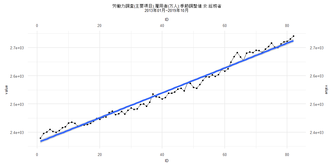
Call:
lm(formula = value ~ ID)

Residuals:
    Min      1Q  Median      3Q     Max
-32.247 -11.196  -2.917  12.144  36.358

Coefficients:
              Estimate Std. Error t value            Pr(>|t|)
(Intercept) 2363.08220    3.45449  684.06 <0.0000000000000002 ***
ID             4.41500    0.07231   61.06 <0.0000000000000002 ***
---
Signif. codes:  0 '***' 0.001 '**' 0.01 '*' 0.05 '.' 0.1 ' ' 1

Residual standard error: 15.5 on 80 degrees of freedom
Multiple R-squared:  0.979, Adjusted R-squared:  0.9787
F-statistic:  3728 on 1 and 80 DF,  p-value: < 0.00000000000000022


    Two-sample Kolmogorov-Smirnov test

data:  lm_residuals and rnorm(n = length(lm_residuals), mean = 0, sd = sd(lm_residuals))
D = 0.13415, p-value = 0.4541
alternative hypothesis: two-sided


    Durbin-Watson test

data:  value ~ ID
DW = 0.39908, p-value < 0.00000000000000022
alternative hypothesis: true autocorrelation is greater than 0


    studentized Breusch-Pagan test

data:  value ~ ID
BP = 0.12991, df = 1, p-value = 0.7185


    Box-Ljung test

data:  lm_residuals
X-squared = 53.132, df = 1, p-value = 0.0000000000003119
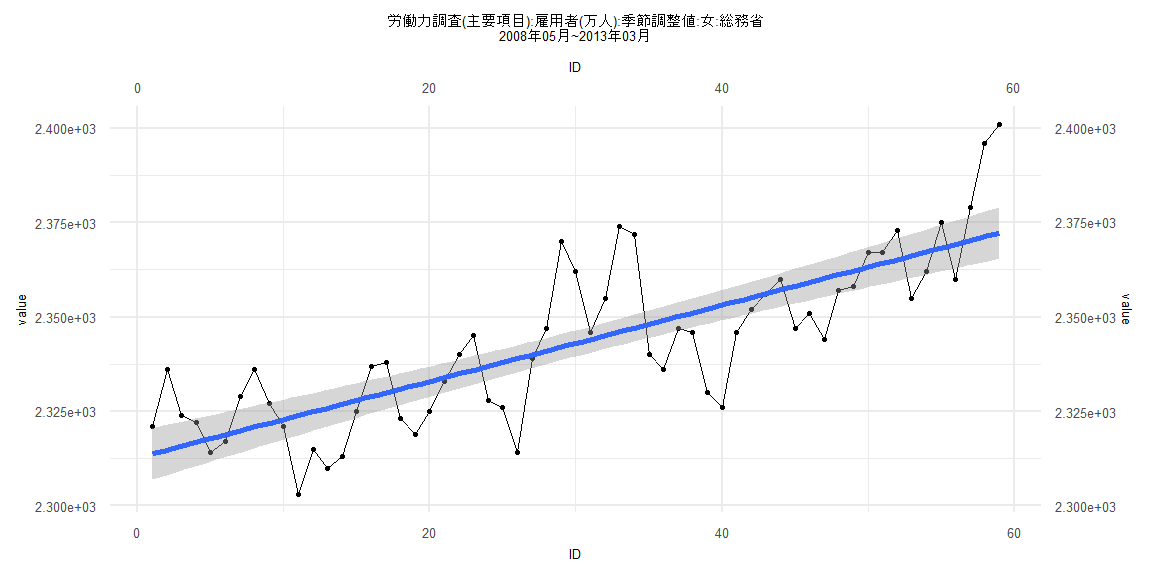
Call:
lm(formula = value ~ ID)

Residuals:
    Min      1Q  Median      3Q     Max
-27.088  -8.544  -1.790   7.960  28.746

Coefficients:
             Estimate Std. Error t value             Pr(>|t|)
(Intercept) 2312.7370     3.4859 663.459 < 0.0000000000000002 ***
ID             1.0088     0.1011   9.983   0.0000000000000401 ***
---
Signif. codes:  0 '***' 0.001 '**' 0.01 '*' 0.05 '.' 0.1 ' ' 1

Residual standard error: 13.22 on 57 degrees of freedom
Multiple R-squared:  0.6361,    Adjusted R-squared:  0.6298
F-statistic: 99.66 on 1 and 57 DF,  p-value: 0.00000000000004005


    Two-sample Kolmogorov-Smirnov test

data:  lm_residuals and rnorm(n = length(lm_residuals), mean = 0, sd = sd(lm_residuals))
D = 0.10169, p-value = 0.9239
alternative hypothesis: two-sided


    Durbin-Watson test

data:  value ~ ID
DW = 0.81794, p-value = 0.00000009453
alternative hypothesis: true autocorrelation is greater than 0


    studentized Breusch-Pagan test

data:  value ~ ID
BP = 0.78708, df = 1, p-value = 0.375


    Box-Ljung test

data:  lm_residuals
X-squared = 18.56, df = 1, p-value = 0.00001647
Call:
lm(formula = value ~ ID)

Residuals:
    Min      1Q  Median      3Q     Max
-31.963 -10.179  -1.869  12.177  35.864

Coefficients:
              Estimate Std. Error t value            Pr(>|t|)
(Intercept) 2373.17137    3.44433  689.01 <0.0000000000000002 ***
ID             4.47483    0.07481   59.82 <0.0000000000000002 ***
---
Signif. codes:  0 '***' 0.001 '**' 0.01 '*' 0.05 '.' 0.1 ' ' 1

Residual standard error: 15.16 on 77 degrees of freedom
Multiple R-squared:  0.9789,    Adjusted R-squared:  0.9787
F-statistic:  3578 on 1 and 77 DF,  p-value: < 0.00000000000000022


    Two-sample Kolmogorov-Smirnov test

data:  lm_residuals and rnorm(n = length(lm_residuals), mean = 0, sd = sd(lm_residuals))
D = 0.088608, p-value = 0.9184
alternative hypothesis: two-sided


    Durbin-Watson test

data:  value ~ ID
DW = 0.42317, p-value < 0.00000000000000022
alternative hypothesis: true autocorrelation is greater than 0


    studentized Breusch-Pagan test

data:  value ~ ID
BP = 0.4779, df = 1, p-value = 0.4894


    Box-Ljung test

data:  lm_residuals
X-squared = 46.523, df = 1, p-value = 0.000000000009054