Analysis
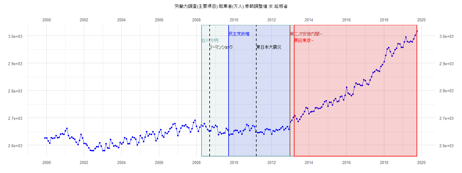
[1] "労働力調査(主要項目):就業者(万人):季節調整値:女:総務省"
      Jan  Feb  Mar  Apr  May  Jun  Jul  Aug  Sep  Oct  Nov  Dec
1999                                                        2627
2000 2627 2616 2608 2628 2626 2627 2635 2628 2629 2641 2642 2640
2001 2653 2662 2635 2626 2630 2626 2622 2611 2602 2618 2640 2627
2002 2607 2606 2600 2590 2582 2581 2581 2588 2595 2595 2609 2597
2003 2581 2581 2606 2590 2589 2621 2608 2597 2599 2596 2592 2610
2004 2605 2610 2628 2623 2606 2606 2621 2630 2628 2622 2601 2610
2005 2636 2627 2614 2630 2650 2634 2641 2640 2650 2641 2617 2624
2006 2649 2658 2636 2630 2647 2643 2650 2661 2665 2677 2680 2661
2007 2635 2650 2663 2672 2671 2675 2667 2664 2649 2661 2684 2692
2008 2670 2651 2666 2674 2671 2679 2668 2657 2652 2653 2668 2665
2009 2673 2669 2639 2648 2642 2644 2645 2662 2656 2638 2641 2641
2010 2653 2655 2654 2646 2652 2641 2654 2659 2676 2672 2654 2662
2011 2672 2669 2649 2647 2646 2649 2648 2641 2657 2661 2657 2657
2012 2641 2653 2651 2658 2655 2657 2663 2668 2656 2662 2668 2659
2013 2685 2691 2702 2708 2697 2687 2695 2705 2714 2723 2738 2735
2014 2716 2722 2723 2724 2737 2738 2734 2735 2740 2750 2760 2763
2015 2743 2757 2758 2748 2764 2771 2760 2762 2777 2779 2766 2783
2016 2813 2791 2787 2782 2787 2814 2828 2823 2823 2819 2819 2840
2017 2837 2825 2822 2839 2851 2866 2870 2876 2873 2871 2888 2895
2018 2906 2929 2952 2958 2943 2927 2937 2950 2955 2972 2971 2959
2019 2959 2978 2996 2980 2977 2981 2979 2989 3003 3018
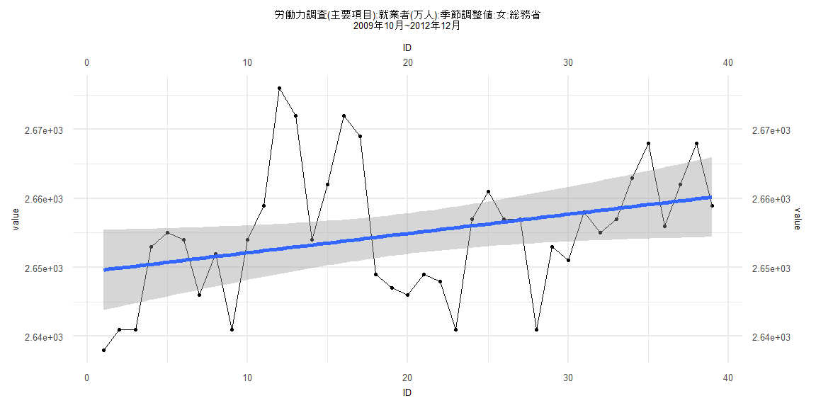
Call:
lm(formula = value ~ ID)

Residuals:
     Min       1Q   Median       3Q      Max
-16.1530  -6.4562   0.1257   4.2163  23.3069

Coefficients:
             Estimate Std. Error t value            Pr(>|t|)
(Intercept) 2649.3482     2.9776 889.767 <0.0000000000000002 ***
ID             0.2787     0.1297   2.148              0.0383 *
---
Signif. codes:  0 '***' 0.001 '**' 0.01 '*' 0.05 '.' 0.1 ' ' 1

Residual standard error: 9.119 on 37 degrees of freedom
Multiple R-squared:  0.1109,    Adjusted R-squared:  0.08688
F-statistic: 4.616 on 1 and 37 DF,  p-value: 0.0383


    Two-sample Kolmogorov-Smirnov test

data:  lm_residuals and rnorm(n = length(lm_residuals), mean = 0, sd = sd(lm_residuals))
D = 0.12821, p-value = 0.9114
alternative hypothesis: two-sided


    Durbin-Watson test

data:  value ~ ID
DW = 0.95623, p-value = 0.00009292
alternative hypothesis: true autocorrelation is greater than 0


    studentized Breusch-Pagan test

data:  value ~ ID
BP = 1.6619, df = 1, p-value = 0.1974


    Box-Ljung test

data:  lm_residuals
X-squared = 10.506, df = 1, p-value = 0.00119
Call:
lm(formula = value ~ ID)

Residuals:
   Min     1Q Median     3Q    Max
-42.58 -15.58   1.56  16.16  40.90

Coefficients:
              Estimate Std. Error t value            Pr(>|t|)
(Intercept) 2658.52846    4.57138  581.56 <0.0000000000000002 ***
ID             4.04016    0.09568   42.22 <0.0000000000000002 ***
---
Signif. codes:  0 '***' 0.001 '**' 0.01 '*' 0.05 '.' 0.1 ' ' 1

Residual standard error: 20.51 on 80 degrees of freedom
Multiple R-squared:  0.9571,    Adjusted R-squared:  0.9565
F-statistic:  1783 on 1 and 80 DF,  p-value: < 0.00000000000000022


    Two-sample Kolmogorov-Smirnov test

data:  lm_residuals and rnorm(n = length(lm_residuals), mean = 0, sd = sd(lm_residuals))
D = 0.073171, p-value = 0.9818
alternative hypothesis: two-sided


    Durbin-Watson test

data:  value ~ ID
DW = 0.30415, p-value < 0.00000000000000022
alternative hypothesis: true autocorrelation is greater than 0


    studentized Breusch-Pagan test

data:  value ~ ID
BP = 0.23809, df = 1, p-value = 0.6256


    Box-Ljung test

data:  lm_residuals
X-squared = 58.391, df = 1, p-value = 0.00000000000002154
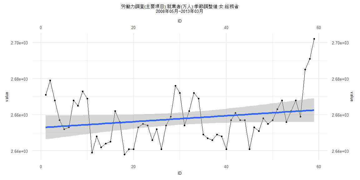
Call:
lm(formula = value ~ ID)

Residuals:
    Min      1Q  Median      3Q     Max
-19.277  -9.881  -2.770   6.530  39.424

Coefficients:
              Estimate Std. Error t value            Pr(>|t|)
(Intercept) 2652.88662    3.40276 779.627 <0.0000000000000002 ***
ID             0.16423    0.09864   1.665               0.101
---
Signif. codes:  0 '***' 0.001 '**' 0.01 '*' 0.05 '.' 0.1 ' ' 1

Residual standard error: 12.9 on 57 degrees of freedom
Multiple R-squared:  0.04638,   Adjusted R-squared:  0.02965
F-statistic: 2.772 on 1 and 57 DF,  p-value: 0.1014


    Two-sample Kolmogorov-Smirnov test

data:  lm_residuals and rnorm(n = length(lm_residuals), mean = 0, sd = sd(lm_residuals))
D = 0.11864, p-value = 0.8052
alternative hypothesis: two-sided


    Durbin-Watson test

data:  value ~ ID
DW = 0.64202, p-value = 0.0000000002414
alternative hypothesis: true autocorrelation is greater than 0


    studentized Breusch-Pagan test

data:  value ~ ID
BP = 0.69705, df = 1, p-value = 0.4038


    Box-Ljung test

data:  lm_residuals
X-squared = 20.883, df = 1, p-value = 0.000004882
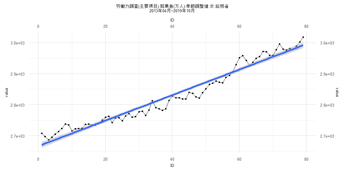
Call:
lm(formula = value ~ ID)

Residuals:
    Min      1Q  Median      3Q     Max
-42.210 -14.673   1.021  12.821  40.257

Coefficients:
              Estimate Std. Error t value            Pr(>|t|)
(Intercept) 2666.54722    4.57588  582.74 <0.0000000000000002 ***
ID             4.11796    0.09938   41.44 <0.0000000000000002 ***
---
Signif. codes:  0 '***' 0.001 '**' 0.01 '*' 0.05 '.' 0.1 ' ' 1

Residual standard error: 20.14 on 77 degrees of freedom
Multiple R-squared:  0.9571,    Adjusted R-squared:  0.9565
F-statistic:  1717 on 1 and 77 DF,  p-value: < 0.00000000000000022


    Two-sample Kolmogorov-Smirnov test

data:  lm_residuals and rnorm(n = length(lm_residuals), mean = 0, sd = sd(lm_residuals))
D = 0.11392, p-value = 0.6878
alternative hypothesis: two-sided


    Durbin-Watson test

data:  value ~ ID
DW = 0.32583, p-value < 0.00000000000000022
alternative hypothesis: true autocorrelation is greater than 0


    studentized Breusch-Pagan test

data:  value ~ ID
BP = 0.0028092, df = 1, p-value = 0.9577


    Box-Ljung test

data:  lm_residuals
X-squared = 53.011, df = 1, p-value = 0.0000000000003317