Analysis
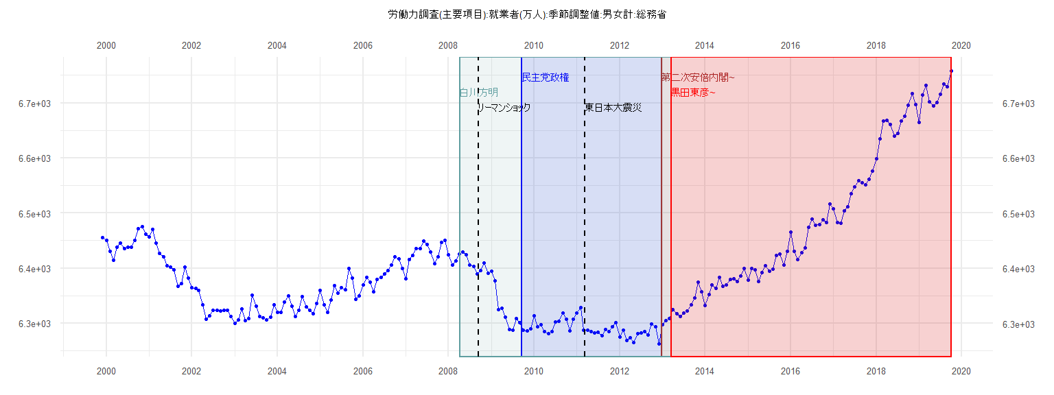
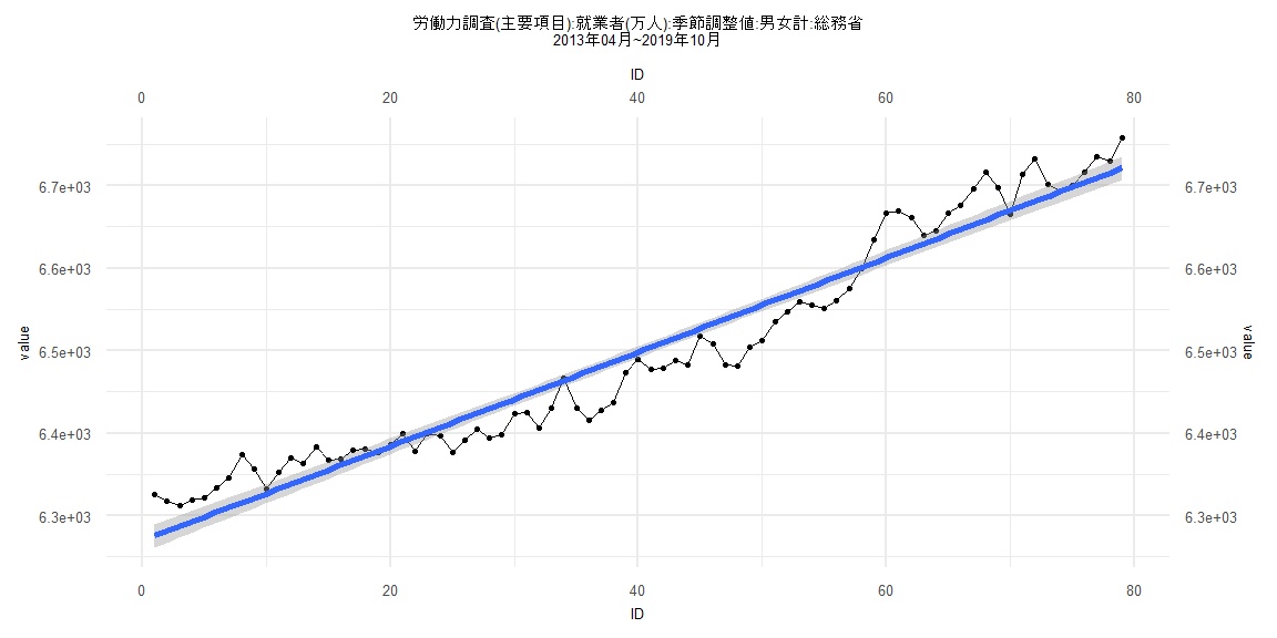
[1] "労働力調査(主要項目):就業者(万人):季節調整値:男女計:総務省"
      Jan  Feb  Mar  Apr  May  Jun  Jul  Aug  Sep  Oct  Nov  Dec
1999                                                        6456
2000 6450 6430 6414 6438 6445 6436 6438 6438 6451 6472 6476 6462
2001 6457 6470 6445 6427 6421 6404 6402 6397 6367 6372 6402 6382
2002 6365 6363 6360 6334 6307 6313 6324 6324 6322 6324 6324 6312
2003 6300 6306 6326 6305 6309 6351 6331 6312 6310 6306 6311 6333
2004 6320 6320 6339 6350 6331 6312 6324 6348 6330 6323 6317 6336
2005 6360 6334 6320 6342 6368 6355 6365 6361 6399 6382 6343 6350
2006 6369 6383 6374 6357 6379 6383 6389 6396 6406 6421 6417 6400
2007 6381 6416 6423 6436 6436 6449 6443 6429 6408 6420 6447 6450
2008 6424 6406 6413 6426 6429 6424 6406 6403 6390 6396 6410 6391
2009 6394 6377 6325 6327 6311 6289 6287 6309 6301 6287 6286 6290
2010 6314 6294 6297 6285 6281 6285 6302 6304 6319 6307 6286 6307
2011 6319 6329 6287 6287 6285 6282 6284 6277 6289 6285 6294 6301
2012 6275 6287 6269 6274 6265 6281 6282 6285 6279 6299 6293 6263
2013 6297 6305 6309 6325 6317 6312 6319 6322 6333 6346 6374 6357
2014 6332 6352 6370 6363 6383 6367 6369 6379 6381 6376 6386 6399
2015 6378 6400 6397 6376 6392 6405 6394 6398 6423 6425 6406 6431
2016 6466 6431 6416 6428 6437 6474 6489 6478 6479 6488 6483 6517
2017 6508 6483 6482 6504 6512 6535 6547 6559 6555 6551 6561 6576
2018 6599 6635 6667 6669 6661 6640 6645 6667 6676 6696 6717 6697
2019 6665 6714 6732 6702 6694 6701 6716 6735 6730 6758
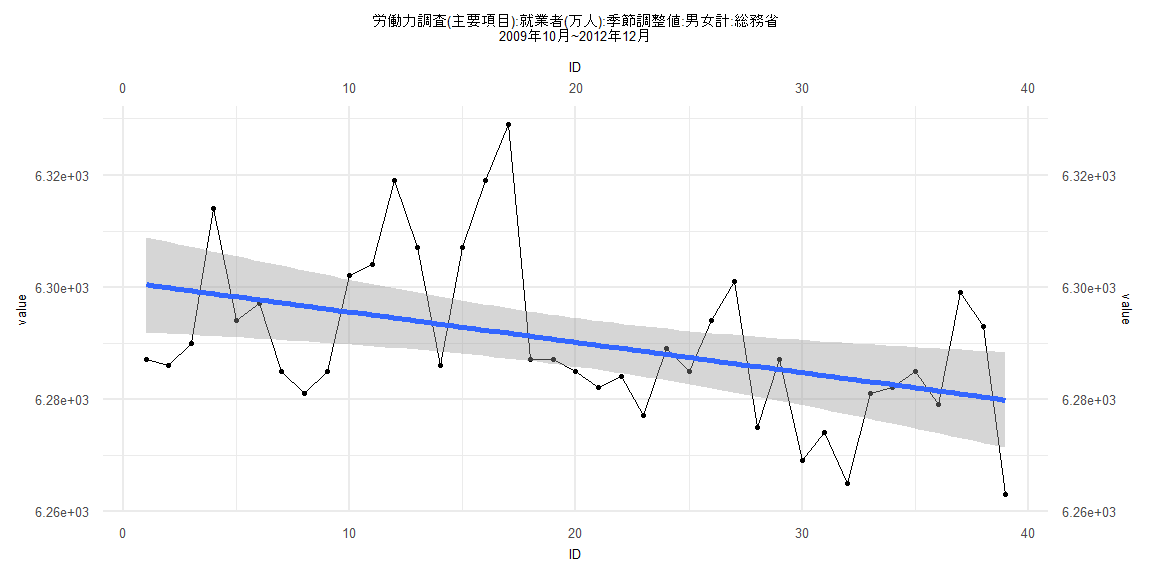
Call:
lm(formula = value ~ ID)

Residuals:
    Min      1Q  Median      3Q     Max
-18.635 -10.488  -2.471   8.060  37.249

Coefficients:
             Estimate Std. Error  t value             Pr(>|t|)
(Intercept) 6300.9501     4.3701 1441.819 < 0.0000000000000002 ***
ID            -0.5411     0.1904   -2.841              0.00726 **
---
Signif. codes:  0 '***' 0.001 '**' 0.01 '*' 0.05 '.' 0.1 ' ' 1

Residual standard error: 13.38 on 37 degrees of freedom
Multiple R-squared:  0.1791,    Adjusted R-squared:  0.1569
F-statistic: 8.074 on 1 and 37 DF,  p-value: 0.007262


    Two-sample Kolmogorov-Smirnov test

data:  lm_residuals and rnorm(n = length(lm_residuals), mean = 0, sd = sd(lm_residuals))
D = 0.15385, p-value = 0.7523
alternative hypothesis: two-sided


    Durbin-Watson test

data:  value ~ ID
DW = 1.2008, p-value = 0.002502
alternative hypothesis: true autocorrelation is greater than 0


    studentized Breusch-Pagan test

data:  value ~ ID
BP = 0.25409, df = 1, p-value = 0.6142


    Box-Ljung test

data:  lm_residuals
X-squared = 5.5939, df = 1, p-value = 0.01802
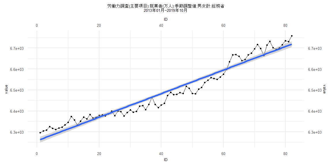
Call:
lm(formula = value ~ ID)

Residuals:
    Min      1Q  Median      3Q     Max
-62.466 -26.041   2.217  27.707  60.256

Coefficients:
             Estimate Std. Error t value            Pr(>|t|)
(Intercept) 6258.1572     7.1355  877.04 <0.0000000000000002 ***
ID             5.6139     0.1494   37.59 <0.0000000000000002 ***
---
Signif. codes:  0 '***' 0.001 '**' 0.01 '*' 0.05 '.' 0.1 ' ' 1

Residual standard error: 32.01 on 80 degrees of freedom
Multiple R-squared:  0.9464,    Adjusted R-squared:  0.9457
F-statistic:  1413 on 1 and 80 DF,  p-value: < 0.00000000000000022


    Two-sample Kolmogorov-Smirnov test

data:  lm_residuals and rnorm(n = length(lm_residuals), mean = 0, sd = sd(lm_residuals))
D = 0.18293, p-value = 0.1288
alternative hypothesis: two-sided


    Durbin-Watson test

data:  value ~ ID
DW = 0.30352, p-value < 0.00000000000000022
alternative hypothesis: true autocorrelation is greater than 0


    studentized Breusch-Pagan test

data:  value ~ ID
BP = 1.364, df = 1, p-value = 0.2429


    Box-Ljung test

data:  lm_residuals
X-squared = 58.863, df = 1, p-value = 0.00000000000001688
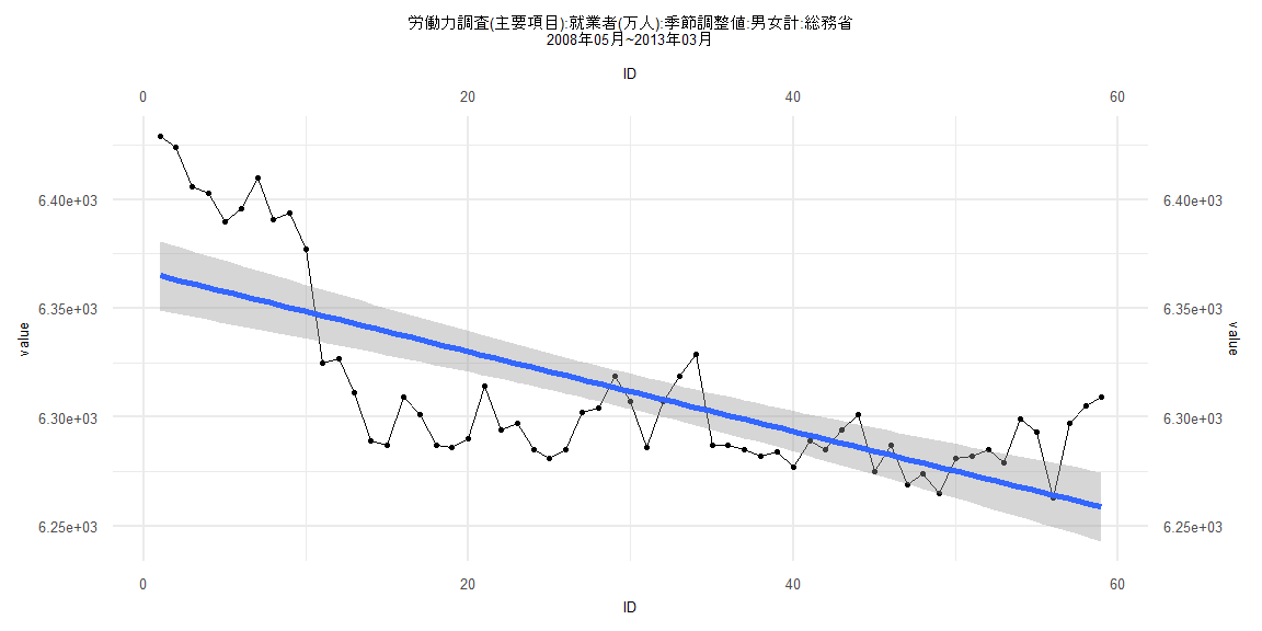
Call:
lm(formula = value ~ ID)

Residuals:
    Min      1Q  Median      3Q     Max
-52.235 -19.641  -4.816  25.760  64.141

Coefficients:
             Estimate Std. Error t value             Pr(>|t|)
(Intercept) 6366.6897     8.1662 779.638 < 0.0000000000000002 ***
ID            -1.8303     0.2367  -7.732       0.000000000192 ***
---
Signif. codes:  0 '***' 0.001 '**' 0.01 '*' 0.05 '.' 0.1 ' ' 1

Residual standard error: 30.97 on 57 degrees of freedom
Multiple R-squared:  0.5119,    Adjusted R-squared:  0.5033
F-statistic: 59.78 on 1 and 57 DF,  p-value: 0.0000000001919


    Two-sample Kolmogorov-Smirnov test

data:  lm_residuals and rnorm(n = length(lm_residuals), mean = 0, sd = sd(lm_residuals))
D = 0.16949, p-value = 0.3674
alternative hypothesis: two-sided


    Durbin-Watson test

data:  value ~ ID
DW = 0.26675, p-value < 0.00000000000000022
alternative hypothesis: true autocorrelation is greater than 0


    studentized Breusch-Pagan test

data:  value ~ ID
BP = 18.361, df = 1, p-value = 0.00001827


    Box-Ljung test

data:  lm_residuals
X-squared = 40.295, df = 1, p-value = 0.0000000002184
Call:
lm(formula = value ~ ID)

Residuals:
    Min      1Q  Median      3Q     Max
-61.985 -26.052   2.046  26.188  58.684

Coefficients:
             Estimate Std. Error t value            Pr(>|t|)
(Intercept) 6269.5920     7.2251  867.75 <0.0000000000000002 ***
ID             5.7165     0.1569   36.43 <0.0000000000000002 ***
---
Signif. codes:  0 '***' 0.001 '**' 0.01 '*' 0.05 '.' 0.1 ' ' 1

Residual standard error: 31.8 on 77 degrees of freedom
Multiple R-squared:  0.9452,    Adjusted R-squared:  0.9444
F-statistic:  1327 on 1 and 77 DF,  p-value: < 0.00000000000000022


    Two-sample Kolmogorov-Smirnov test

data:  lm_residuals and rnorm(n = length(lm_residuals), mean = 0, sd = sd(lm_residuals))
D = 0.11392, p-value = 0.6878
alternative hypothesis: two-sided


    Durbin-Watson test

data:  value ~ ID
DW = 0.31801, p-value < 0.00000000000000022
alternative hypothesis: true autocorrelation is greater than 0


    studentized Breusch-Pagan test

data:  value ~ ID
BP = 0.27202, df = 1, p-value = 0.602


    Box-Ljung test

data:  lm_residuals
X-squared = 54.686, df = 1, p-value = 0.0000000000001414