Analysis
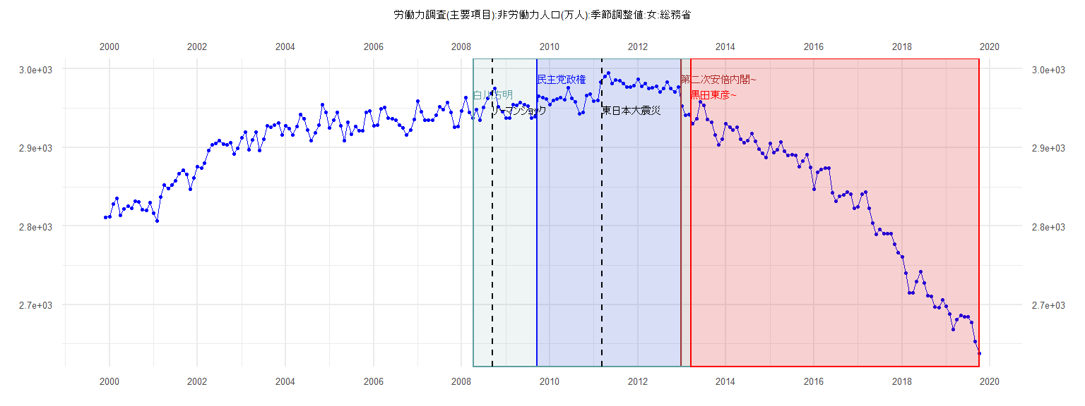
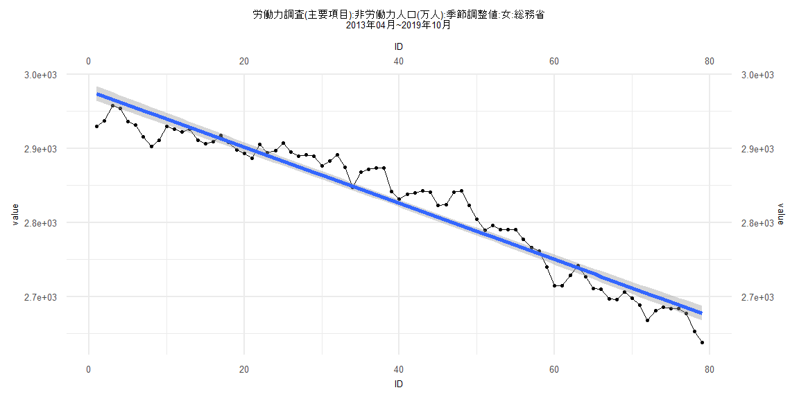
[1] "労働力調査(主要項目):非労働力人口(万人):季節調整値:女:総務省"
      Jan  Feb  Mar  Apr  May  Jun  Jul  Aug  Sep  Oct  Nov  Dec
1999                                                        2811
2000 2812 2828 2835 2814 2822 2825 2823 2832 2831 2821 2820 2830
2001 2816 2806 2837 2852 2848 2852 2858 2867 2871 2866 2847 2861
2002 2876 2874 2880 2896 2903 2905 2909 2904 2903 2906 2892 2899
2003 2912 2920 2897 2910 2920 2896 2911 2928 2926 2929 2931 2916
2004 2928 2924 2916 2927 2942 2937 2922 2909 2919 2929 2955 2945
2005 2925 2935 2945 2928 2909 2932 2917 2927 2921 2921 2945 2947
2006 2928 2929 2949 2951 2938 2937 2935 2929 2925 2916 2922 2936
2007 2959 2946 2935 2935 2935 2941 2952 2948 2957 2945 2926 2927
2008 2947 2964 2945 2938 2948 2935 2951 2963 2969 2975 2952 2946
2009 2938 2938 2955 2954 2957 2955 2953 2938 2939 2965 2964 2962
2010 2955 2960 2962 2964 2961 2976 2963 2958 2943 2945 2966 2968
2011 2959 2960 2983 2991 2995 2982 2986 2985 2982 2977 2977 2979
2012 2987 2978 2982 2975 2976 2978 2971 2975 2983 2975 2971 2977
2013 2953 2941 2942 2930 2937 2958 2954 2936 2932 2916 2903 2911
2014 2930 2926 2922 2926 2911 2906 2909 2918 2908 2898 2893 2887
2015 2905 2894 2897 2907 2895 2890 2891 2890 2876 2883 2891 2875
2016 2847 2868 2872 2874 2874 2842 2832 2838 2840 2843 2841 2823
2017 2824 2841 2843 2823 2804 2789 2796 2790 2790 2790 2777 2766
2018 2761 2740 2715 2715 2729 2742 2727 2711 2710 2697 2696 2706
2019 2698 2688 2668 2681 2686 2684 2684 2677 2653 2638
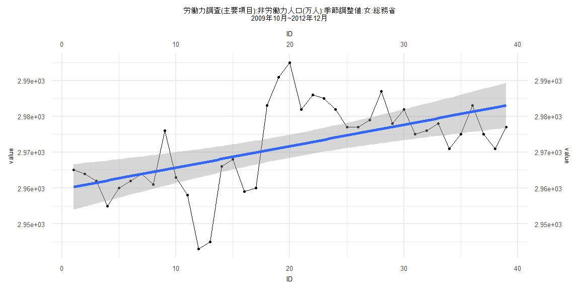
Call:
lm(formula = value ~ ID)

Residuals:
     Min       1Q   Median       3Q      Max
-23.8988  -5.8785  -0.6964   4.5040  23.3077

Coefficients:
             Estimate Std. Error t value             Pr(>|t|)
(Intercept) 2959.7085     3.2407 913.302 < 0.0000000000000002 ***
ID             0.5992     0.1412   4.243             0.000142 ***
---
Signif. codes:  0 '***' 0.001 '**' 0.01 '*' 0.05 '.' 0.1 ' ' 1

Residual standard error: 9.925 on 37 degrees of freedom
Multiple R-squared:  0.3273,    Adjusted R-squared:  0.3092
F-statistic: 18.01 on 1 and 37 DF,  p-value: 0.0001416


    Two-sample Kolmogorov-Smirnov test

data:  lm_residuals and rnorm(n = length(lm_residuals), mean = 0, sd = sd(lm_residuals))
D = 0.12821, p-value = 0.9114
alternative hypothesis: two-sided


    Durbin-Watson test

data:  value ~ ID
DW = 0.70328, p-value = 0.0000006222
alternative hypothesis: true autocorrelation is greater than 0


    studentized Breusch-Pagan test

data:  value ~ ID
BP = 0.24399, df = 1, p-value = 0.6213


    Box-Ljung test

data:  lm_residuals
X-squared = 17.25, df = 1, p-value = 0.00003277
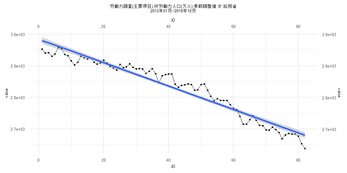
Call:
lm(formula = value ~ ID)

Residuals:
   Min     1Q Median     3Q    Max
-42.00 -17.49  -1.83  17.17  48.05

Coefficients:
             Estimate Std. Error t value            Pr(>|t|)
(Intercept) 2984.0506     5.0865  586.66 <0.0000000000000002 ***
ID            -3.7079     0.1065  -34.83 <0.0000000000000002 ***
---
Signif. codes:  0 '***' 0.001 '**' 0.01 '*' 0.05 '.' 0.1 ' ' 1

Residual standard error: 22.82 on 80 degrees of freedom
Multiple R-squared:  0.9381,    Adjusted R-squared:  0.9374
F-statistic:  1213 on 1 and 80 DF,  p-value: < 0.00000000000000022


    Two-sample Kolmogorov-Smirnov test

data:  lm_residuals and rnorm(n = length(lm_residuals), mean = 0, sd = sd(lm_residuals))
D = 0.060976, p-value = 0.9983
alternative hypothesis: two-sided


    Durbin-Watson test

data:  value ~ ID
DW = 0.26219, p-value < 0.00000000000000022
alternative hypothesis: true autocorrelation is greater than 0


    studentized Breusch-Pagan test

data:  value ~ ID
BP = 0.03038, df = 1, p-value = 0.8616


    Box-Ljung test

data:  lm_residuals
X-squared = 59.825, df = 1, p-value = 0.00000000000001033
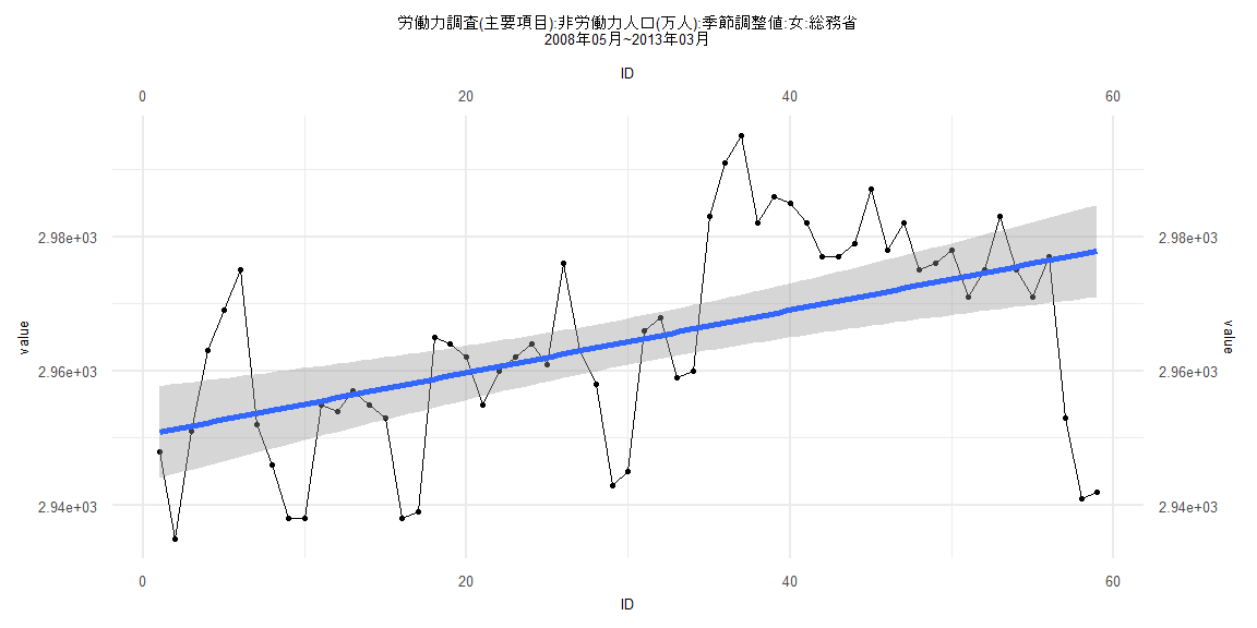
Call:
lm(formula = value ~ ID)

Residuals:
    Min      1Q  Median      3Q     Max
-36.384  -5.090   0.527   7.495  27.374

Coefficients:
             Estimate Std. Error t value             Pr(>|t|)
(Intercept) 2950.4319     3.5145 839.500 < 0.0000000000000002 ***
ID             0.4647     0.1019   4.561            0.0000275 ***
---
Signif. codes:  0 '***' 0.001 '**' 0.01 '*' 0.05 '.' 0.1 ' ' 1

Residual standard error: 13.33 on 57 degrees of freedom
Multiple R-squared:  0.2674,    Adjusted R-squared:  0.2545
F-statistic:  20.8 on 1 and 57 DF,  p-value: 0.00002748


    Two-sample Kolmogorov-Smirnov test

data:  lm_residuals and rnorm(n = length(lm_residuals), mean = 0, sd = sd(lm_residuals))
D = 0.20339, p-value = 0.1748
alternative hypothesis: two-sided


    Durbin-Watson test

data:  value ~ ID
DW = 0.57119, p-value = 0.00000000001175
alternative hypothesis: true autocorrelation is greater than 0


    studentized Breusch-Pagan test

data:  value ~ ID
BP = 3.2176, df = 1, p-value = 0.07285


    Box-Ljung test

data:  lm_residuals
X-squared = 26.258, df = 1, p-value = 0.0000002986
Call:
lm(formula = value ~ ID)

Residuals:
    Min      1Q  Median      3Q     Max
-44.448 -13.694  -1.607  16.214  47.615

Coefficients:
             Estimate Std. Error t value            Pr(>|t|)
(Intercept) 2977.8608     5.0608  588.42 <0.0000000000000002 ***
ID            -3.8016     0.1099  -34.59 <0.0000000000000002 ***
---
Signif. codes:  0 '***' 0.001 '**' 0.01 '*' 0.05 '.' 0.1 ' ' 1

Residual standard error: 22.28 on 77 degrees of freedom
Multiple R-squared:  0.9395,    Adjusted R-squared:  0.9387
F-statistic:  1196 on 1 and 77 DF,  p-value: < 0.00000000000000022


    Two-sample Kolmogorov-Smirnov test

data:  lm_residuals and rnorm(n = length(lm_residuals), mean = 0, sd = sd(lm_residuals))
D = 0.16456, p-value = 0.2361
alternative hypothesis: two-sided


    Durbin-Watson test

data:  value ~ ID
DW = 0.28166, p-value < 0.00000000000000022
alternative hypothesis: true autocorrelation is greater than 0


    studentized Breusch-Pagan test

data:  value ~ ID
BP = 0.090874, df = 1, p-value = 0.7631


    Box-Ljung test

data:  lm_residuals
X-squared = 54.267, df = 1, p-value = 0.000000000000175