Analysis
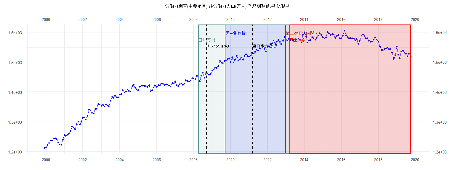
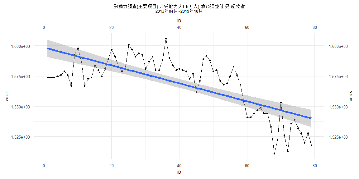
[1] "労働力調査(主要項目):非労働力人口(万人):季節調整値:男:総務省"
      Jan  Feb  Mar  Apr  May  Jun  Jul  Aug  Sep  Oct  Nov  Dec
1999                                                        1213
2000 1216 1222 1229 1237 1237 1244 1245 1242 1231 1224 1223 1240
2001 1256 1253 1257 1260 1270 1285 1281 1276 1293 1302 1292 1301
2002 1315 1314 1308 1320 1341 1338 1330 1328 1343 1344 1360 1358
2003 1354 1357 1352 1358 1355 1353 1372 1384 1381 1388 1383 1382
2004 1392 1393 1406 1398 1401 1408 1403 1401 1420 1424 1414 1409
2005 1405 1418 1422 1421 1420 1420 1417 1423 1402 1405 1415 1421
2006 1417 1423 1422 1429 1428 1423 1426 1425 1422 1418 1430 1429
2007 1436 1422 1420 1426 1429 1424 1428 1440 1437 1435 1439 1447
2008 1446 1443 1455 1447 1436 1455 1466 1448 1464 1463 1458 1461
2009 1472 1476 1482 1480 1485 1504 1498 1497 1504 1506 1510 1513
2010 1500 1517 1499 1510 1521 1506 1509 1516 1508 1521 1527 1521
2011 1519 1522 1532 1529 1535 1542 1539 1547 1557 1558 1545 1536
2012 1552 1552 1561 1564 1572 1561 1568 1574 1568 1560 1571 1584
2013 1574 1572 1578 1574 1574 1574 1575 1576 1579 1576 1567 1593
2014 1598 1587 1567 1573 1574 1584 1580 1575 1581 1589 1597 1591
2015 1583 1579 1583 1601 1597 1591 1594 1593 1581 1587 1591 1580
2016 1580 1588 1606 1590 1584 1580 1581 1580 1579 1573 1577 1562
2017 1571 1589 1592 1588 1579 1580 1571 1568 1569 1575 1583 1576
2018 1568 1554 1541 1541 1544 1547 1549 1544 1544 1533 1511 1522
2019 1553 1526 1513 1536 1539 1532 1528 1520 1528 1518
Call:
lm(formula = value ~ ID)

Residuals:
    Min      1Q  Median      3Q     Max
-14.957  -4.859  -1.265   5.837  12.145

Coefficients:
             Estimate Std. Error t value            Pr(>|t|)
(Intercept) 1496.0337     2.4458  611.66 <0.0000000000000002 ***
ID             2.0342     0.1066   19.09 <0.0000000000000002 ***
---
Signif. codes:  0 '***' 0.001 '**' 0.01 '*' 0.05 '.' 0.1 ' ' 1

Residual standard error: 7.491 on 37 degrees of freedom
Multiple R-squared:  0.9078,    Adjusted R-squared:  0.9053
F-statistic: 364.3 on 1 and 37 DF,  p-value: < 0.00000000000000022


    Two-sample Kolmogorov-Smirnov test

data:  lm_residuals and rnorm(n = length(lm_residuals), mean = 0, sd = sd(lm_residuals))
D = 0.17949, p-value = 0.5622
alternative hypothesis: two-sided


    Durbin-Watson test

data:  value ~ ID
DW = 1.4999, p-value = 0.03787
alternative hypothesis: true autocorrelation is greater than 0


    studentized Breusch-Pagan test

data:  value ~ ID
BP = 0.63825, df = 1, p-value = 0.4243


    Box-Ljung test

data:  lm_residuals
X-squared = 1.9808, df = 1, p-value = 0.1593
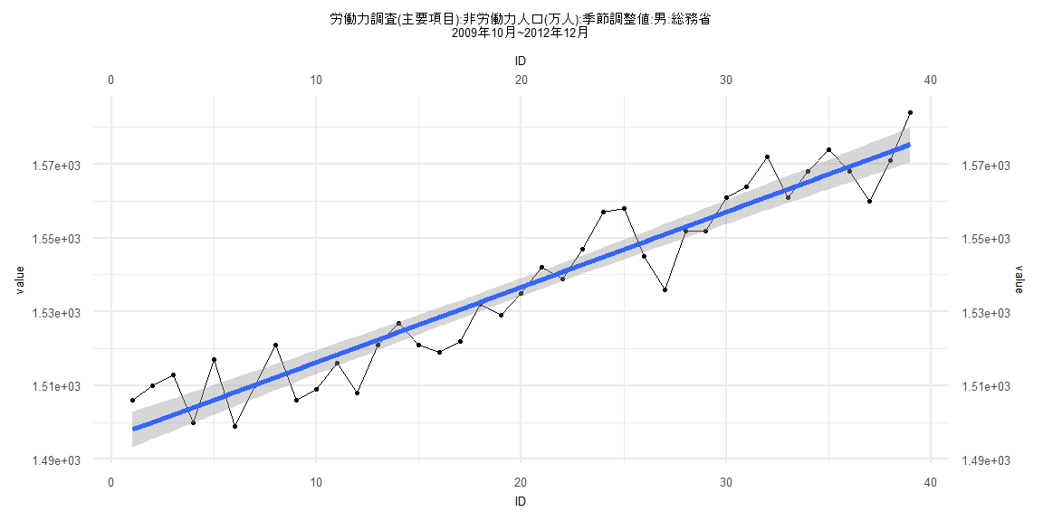
Call:
lm(formula = value ~ ID)

Residuals:
    Min      1Q  Median      3Q     Max
-38.282 -13.663   0.892  12.594  35.038

Coefficients:
              Estimate Std. Error t value             Pr(>|t|)
(Intercept) 1597.38482    3.67028 435.221 < 0.0000000000000002 ***
ID            -0.67751    0.07682  -8.819    0.000000000000199 ***
---
Signif. codes:  0 '***' 0.001 '**' 0.01 '*' 0.05 '.' 0.1 ' ' 1

Residual standard error: 16.47 on 80 degrees of freedom
Multiple R-squared:  0.4929,    Adjusted R-squared:  0.4866
F-statistic: 77.77 on 1 and 80 DF,  p-value: 0.0000000000001993


    Two-sample Kolmogorov-Smirnov test

data:  lm_residuals and rnorm(n = length(lm_residuals), mean = 0, sd = sd(lm_residuals))
D = 0.12195, p-value = 0.5785
alternative hypothesis: two-sided


    Durbin-Watson test

data:  value ~ ID
DW = 0.37515, p-value < 0.00000000000000022
alternative hypothesis: true autocorrelation is greater than 0


    studentized Breusch-Pagan test

data:  value ~ ID
BP = 1.2536, df = 1, p-value = 0.2629


    Box-Ljung test

data:  lm_residuals
X-squared = 52.729, df = 1, p-value = 0.0000000000003828
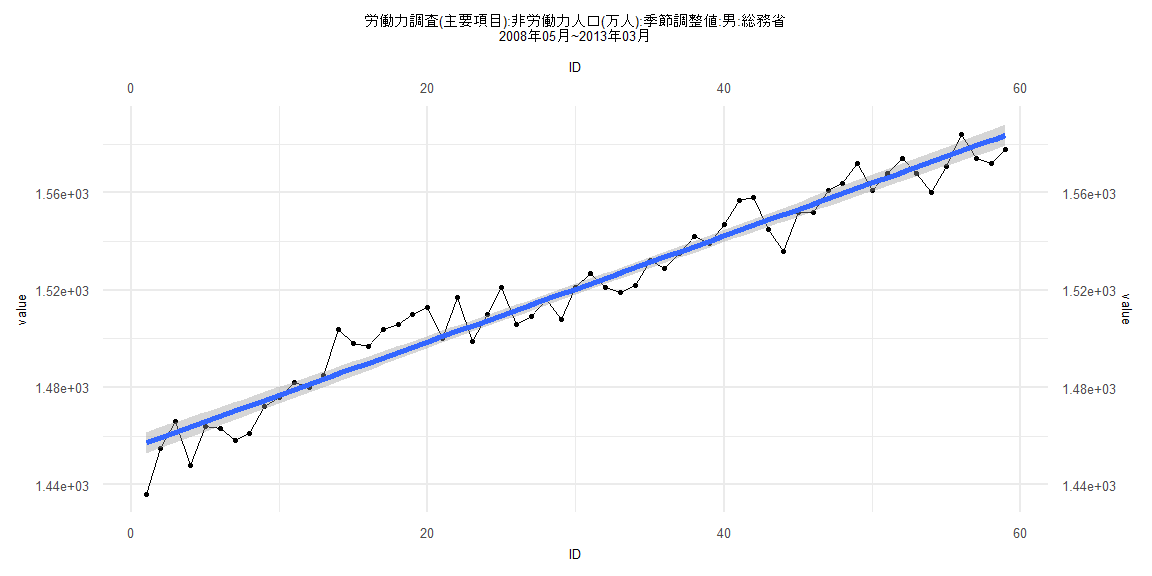
Call:
lm(formula = value ~ ID)

Residuals:
     Min       1Q   Median       3Q      Max
-21.1559  -4.9715  -0.7908   4.6203  18.4826

Coefficients:
              Estimate Std. Error t value            Pr(>|t|)
(Intercept) 1454.97428    2.23117  652.11 <0.0000000000000002 ***
ID             2.18165    0.06468   33.73 <0.0000000000000002 ***
---
Signif. codes:  0 '***' 0.001 '**' 0.01 '*' 0.05 '.' 0.1 ' ' 1

Residual standard error: 8.46 on 57 degrees of freedom
Multiple R-squared:  0.9523,    Adjusted R-squared:  0.9515
F-statistic:  1138 on 1 and 57 DF,  p-value: < 0.00000000000000022


    Two-sample Kolmogorov-Smirnov test

data:  lm_residuals and rnorm(n = length(lm_residuals), mean = 0, sd = sd(lm_residuals))
D = 0.084746, p-value = 0.9854
alternative hypothesis: two-sided


    Durbin-Watson test

data:  value ~ ID
DW = 1.1815, p-value = 0.0002833
alternative hypothesis: true autocorrelation is greater than 0


    studentized Breusch-Pagan test

data:  value ~ ID
BP = 4.4038, df = 1, p-value = 0.03586


    Box-Ljung test

data:  lm_residuals
X-squared = 7.6192, df = 1, p-value = 0.005775
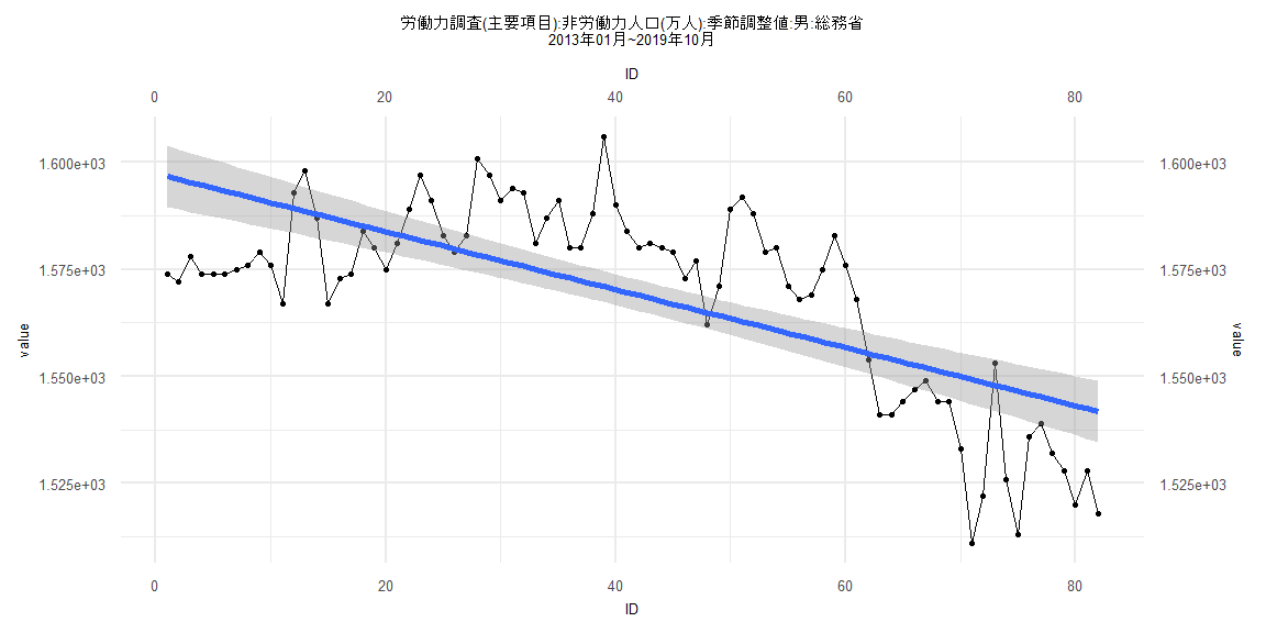
Call:
lm(formula = value ~ ID)

Residuals:
    Min      1Q  Median      3Q     Max
-37.298 -13.057   0.947  12.111  33.970

Coefficients:
              Estimate Std. Error t value             Pr(>|t|)
(Intercept) 1598.72736    3.66812 435.844 < 0.0000000000000002 ***
ID            -0.74160    0.07967  -9.309   0.0000000000000305 ***
---
Signif. codes:  0 '***' 0.001 '**' 0.01 '*' 0.05 '.' 0.1 ' ' 1

Residual standard error: 16.15 on 77 degrees of freedom
Multiple R-squared:  0.5295,    Adjusted R-squared:  0.5234
F-statistic: 86.65 on 1 and 77 DF,  p-value: 0.0000000000000305


    Two-sample Kolmogorov-Smirnov test

data:  lm_residuals and rnorm(n = length(lm_residuals), mean = 0, sd = sd(lm_residuals))
D = 0.12658, p-value = 0.5543
alternative hypothesis: two-sided


    Durbin-Watson test

data:  value ~ ID
DW = 0.40247, p-value < 0.00000000000000022
alternative hypothesis: true autocorrelation is greater than 0


    studentized Breusch-Pagan test

data:  value ~ ID
BP = 0.42471, df = 1, p-value = 0.5146


    Box-Ljung test

data:  lm_residuals
X-squared = 48.923, df = 1, p-value = 0.000000000002663