Analysis
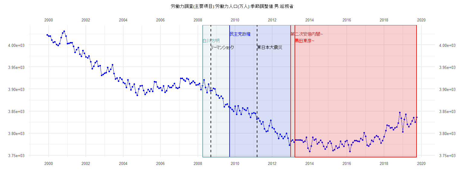
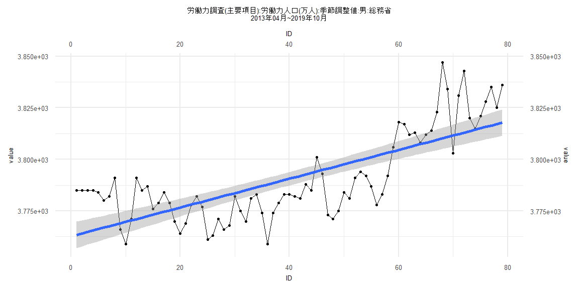
[1] "労働力調査(主要項目):労働力人口(万人):季節調整値:男:総務省"
      Jan  Feb  Mar  Apr  May  Jun  Jul  Aug  Sep  Oct  Nov  Dec
1999                                                        4023
2000 4020 4020 4011 4006 4007 4001 3999 4003 4017 4027 4031 4020
2001 4003 4004 4005 4005 3997 3983 3989 3994 3979 3974 3987 3981
2002 3973 3971 3975 3962 3946 3952 3960 3963 3952 3953 3931 3933
2003 3936 3937 3949 3940 3945 3955 3935 3923 3925 3918 3926 3922
2004 3915 3913 3904 3921 3912 3898 3905 3911 3892 3886 3900 3907
2005 3908 3897 3888 3892 3899 3895 3900 3895 3917 3916 3905 3902
2006 3903 3897 3907 3893 3896 3907 3904 3904 3908 3913 3903 3902
2007 3904 3924 3924 3921 3918 3924 3922 3912 3915 3918 3915 3909
2008 3910 3913 3899 3908 3921 3904 3892 3911 3896 3897 3902 3900
2009 3887 3885 3880 3884 3879 3860 3865 3866 3860 3858 3854 3850
2010 3861 3843 3862 3851 3843 3857 3854 3852 3857 3844 3836 3845
2011 3846 3845 3832 3834 3828 3821 3826 3810 3804 3805 3817 3829
2012 3813 3810 3803 3800 3788 3798 3793 3788 3792 3800 3789 3773
2013 3782 3785 3780 3785 3785 3785 3785 3784 3780 3782 3791 3766
2014 3759 3771 3791 3785 3787 3776 3779 3784 3779 3770 3764 3769
2015 3778 3782 3777 3761 3763 3771 3766 3768 3782 3775 3770 3781
2016 3783 3774 3759 3774 3779 3783 3783 3782 3781 3788 3785 3801
2017 3793 3773 3771 3775 3784 3781 3791 3794 3792 3787 3778 3783
2018 3792 3806 3818 3817 3812 3813 3808 3812 3814 3823 3847 3834
2019 3803 3831 3843 3820 3815 3821 3828 3835 3825 3836
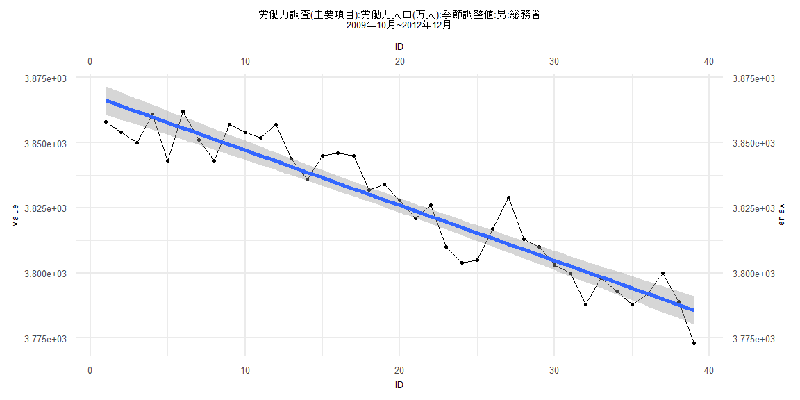
Call:
lm(formula = value ~ ID)

Residuals:
    Min      1Q  Median      3Q     Max
-14.693  -7.159   1.189   6.192  17.903

Coefficients:
            Estimate Std. Error t value            Pr(>|t|)
(Intercept) 3868.283      2.777  1393.1 <0.0000000000000002 ***
ID            -2.118      0.121   -17.5 <0.0000000000000002 ***
---
Signif. codes:  0 '***' 0.001 '**' 0.01 '*' 0.05 '.' 0.1 ' ' 1

Residual standard error: 8.504 on 37 degrees of freedom
Multiple R-squared:  0.8923,    Adjusted R-squared:  0.8893
F-statistic: 306.4 on 1 and 37 DF,  p-value: < 0.00000000000000022


    Two-sample Kolmogorov-Smirnov test

data:  lm_residuals and rnorm(n = length(lm_residuals), mean = 0, sd = sd(lm_residuals))
D = 0.15385, p-value = 0.7523
alternative hypothesis: two-sided


    Durbin-Watson test

data:  value ~ ID
DW = 1.2412, p-value = 0.003882
alternative hypothesis: true autocorrelation is greater than 0


    studentized Breusch-Pagan test

data:  value ~ ID
BP = 0.39684, df = 1, p-value = 0.5287


    Box-Ljung test

data:  lm_residuals
X-squared = 4.776, df = 1, p-value = 0.02886
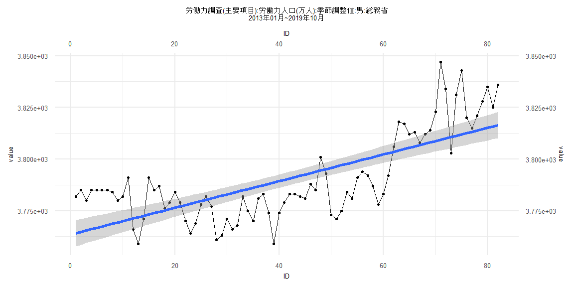
Call:
lm(formula = value ~ ID)

Residuals:
    Min      1Q  Median      3Q     Max
-29.692 -10.959  -1.609  12.138  37.659

Coefficients:
              Estimate Std. Error  t value             Pr(>|t|)
(Intercept) 3763.52575    3.25638 1155.740 < 0.0000000000000002 ***
ID             0.64528    0.06816    9.467   0.0000000000000106 ***
---
Signif. codes:  0 '***' 0.001 '**' 0.01 '*' 0.05 '.' 0.1 ' ' 1

Residual standard error: 14.61 on 80 degrees of freedom
Multiple R-squared:  0.5284,    Adjusted R-squared:  0.5225
F-statistic: 89.63 on 1 and 80 DF,  p-value: 0.00000000000001064


    Two-sample Kolmogorov-Smirnov test

data:  lm_residuals and rnorm(n = length(lm_residuals), mean = 0, sd = sd(lm_residuals))
D = 0.14634, p-value = 0.3453
alternative hypothesis: two-sided


    Durbin-Watson test

data:  value ~ ID
DW = 0.49185, p-value < 0.00000000000000022
alternative hypothesis: true autocorrelation is greater than 0


    studentized Breusch-Pagan test

data:  value ~ ID
BP = 0.97185, df = 1, p-value = 0.3242


    Box-Ljung test

data:  lm_residuals
X-squared = 45.759, df = 1, p-value = 0.00000000001337
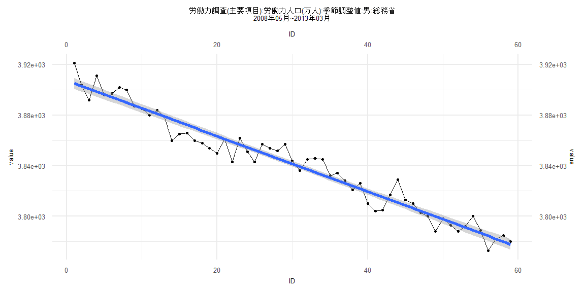
Call:
lm(formula = value ~ ID)

Residuals:
     Min       1Q   Median       3Q      Max
-16.5212  -5.7129   0.3337   5.0248  18.1912

Coefficients:
              Estimate Std. Error t value            Pr(>|t|)
(Intercept) 3907.18703    2.19714 1778.31 <0.0000000000000002 ***
ID            -2.19041    0.06369  -34.39 <0.0000000000000002 ***
---
Signif. codes:  0 '***' 0.001 '**' 0.01 '*' 0.05 '.' 0.1 ' ' 1

Residual standard error: 8.331 on 57 degrees of freedom
Multiple R-squared:  0.954, Adjusted R-squared:  0.9532
F-statistic:  1183 on 1 and 57 DF,  p-value: < 0.00000000000000022


    Two-sample Kolmogorov-Smirnov test

data:  lm_residuals and rnorm(n = length(lm_residuals), mean = 0, sd = sd(lm_residuals))
D = 0.18644, p-value = 0.2582
alternative hypothesis: two-sided


    Durbin-Watson test

data:  value ~ ID
DW = 1.2642, p-value = 0.001018
alternative hypothesis: true autocorrelation is greater than 0


    studentized Breusch-Pagan test

data:  value ~ ID
BP = 1.3631, df = 1, p-value = 0.243


    Box-Ljung test

data:  lm_residuals
X-squared = 6.964, df = 1, p-value = 0.008317
Call:
lm(formula = value ~ ID)

Residuals:
   Min     1Q Median     3Q    Max
-28.82 -10.61  -1.63  12.01  36.85

Coefficients:
             Estimate Std. Error  t value             Pr(>|t|)
(Intercept) 3762.6952     3.2736 1149.410 < 0.0000000000000002 ***
ID             0.6978     0.0711    9.815  0.00000000000000326 ***
---
Signif. codes:  0 '***' 0.001 '**' 0.01 '*' 0.05 '.' 0.1 ' ' 1

Residual standard error: 14.41 on 77 degrees of freedom
Multiple R-squared:  0.5558,    Adjusted R-squared:   0.55
F-statistic: 96.33 on 1 and 77 DF,  p-value: 0.000000000000003264


    Two-sample Kolmogorov-Smirnov test

data:  lm_residuals and rnorm(n = length(lm_residuals), mean = 0, sd = sd(lm_residuals))
D = 0.088608, p-value = 0.9184
alternative hypothesis: two-sided


    Durbin-Watson test

data:  value ~ ID
DW = 0.52171, p-value = 0.0000000000000003647
alternative hypothesis: true autocorrelation is greater than 0


    studentized Breusch-Pagan test

data:  value ~ ID
BP = 0.27656, df = 1, p-value = 0.599


    Box-Ljung test

data:  lm_residuals
X-squared = 41.848, df = 1, p-value = 0.00000000009865