Analysis
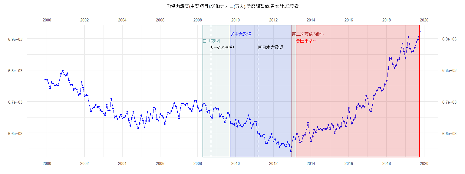
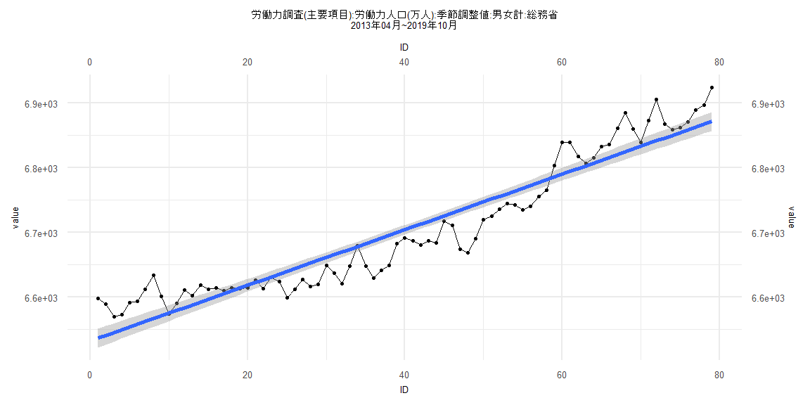
[1] "労働力調査(主要項目):労働力人口(万人):季節調整値:男女計:総務省"
      Jan  Feb  Mar  Apr  May  Jun  Jul  Aug  Sep  Oct  Nov  Dec
1999                                                        6770
2000 6769 6759 6742 6763 6758 6752 6754 6752 6768 6789 6798 6787
2001 6783 6790 6767 6754 6755 6738 6742 6739 6721 6725 6765 6745
2002 6716 6721 6719 6688 6669 6678 6682 6690 6683 6684 6673 6669
2003 6663 6656 6691 6672 6672 6710 6678 6649 6654 6645 6651 6659
2004 6646 6650 6655 6668 6640 6623 6648 6668 6638 6627 6615 6632
2005 6657 6640 6618 6639 6667 6639 6661 6648 6681 6678 6644 6640
2006 6661 6656 6650 6629 6651 6666 6663 6670 6680 6695 6685 6667
2007 6646 6681 6694 6694 6690 6694 6682 6677 6670 6686 6703 6702
2008 6683 6669 6672 6690 6694 6689 6667 6672 6653 6648 6676 6681
2009 6677 6677 6652 6660 6652 6634 6646 6666 6658 6631 6630 6626
2010 6643 6620 6639 6625 6620 6625 6631 6638 6657 6643 6616 6626
2011 6637 6637 6601 6597 6591 6592 6595 6568 6568 6577 6588 6597
2012 6573 6581 6567 6571 6556 6566 6567 6562 6557 6571 6563 6542
2013 6576 6588 6581 6598 6589 6570 6573 6592 6594 6612 6634 6601
2014 6574 6591 6611 6603 6619 6612 6615 6610 6615 6613 6614 6626
2015 6613 6631 6624 6599 6612 6628 6617 6620 6649 6637 6621 6648
2016 6680 6648 6630 6642 6649 6683 6692 6687 6681 6687 6684 6718
2017 6711 6674 6669 6690 6720 6725 6736 6745 6743 6735 6740 6756
2018 6766 6804 6839 6839 6818 6807 6815 6833 6836 6861 6885 6860
2019 6839 6873 6906 6868 6859 6862 6871 6889 6897 6924
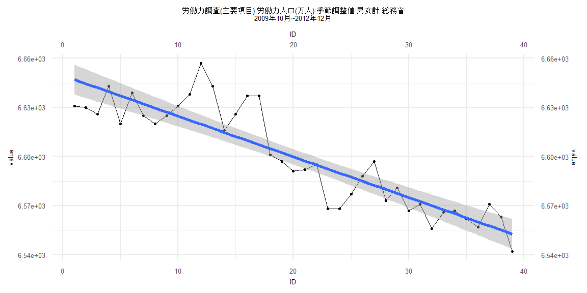
Call:
lm(formula = value ~ ID)

Residuals:
    Min      1Q  Median      3Q     Max
-24.392  -9.255  -1.544   5.336  37.275

Coefficients:
            Estimate Std. Error t value             Pr(>|t|)
(Intercept) 6649.542      4.681 1420.40 < 0.0000000000000002 ***
ID            -2.485      0.204  -12.18   0.0000000000000163 ***
---
Signif. codes:  0 '***' 0.001 '**' 0.01 '*' 0.05 '.' 0.1 ' ' 1

Residual standard error: 14.34 on 37 degrees of freedom
Multiple R-squared:  0.8004,    Adjusted R-squared:  0.795
F-statistic: 148.4 on 1 and 37 DF,  p-value: 0.00000000000001634


    Two-sample Kolmogorov-Smirnov test

data:  lm_residuals and rnorm(n = length(lm_residuals), mean = 0, sd = sd(lm_residuals))
D = 0.12821, p-value = 0.9114
alternative hypothesis: two-sided


    Durbin-Watson test

data:  value ~ ID
DW = 0.93681, p-value = 0.00006772
alternative hypothesis: true autocorrelation is greater than 0


    studentized Breusch-Pagan test

data:  value ~ ID
BP = 1.9822, df = 1, p-value = 0.1592


    Box-Ljung test

data:  lm_residuals
X-squared = 10.825, df = 1, p-value = 0.001001
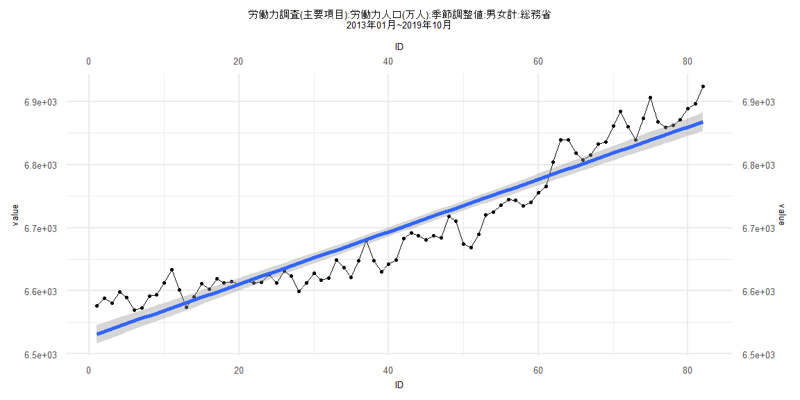
Call:
lm(formula = value ~ ID)

Residuals:
    Min      1Q  Median      3Q     Max
-70.312 -26.094  -0.785  23.591  66.941

Coefficients:
             Estimate Std. Error t value            Pr(>|t|)
(Intercept) 6527.3505     7.5116  868.98 <0.0000000000000002 ***
ID             4.1561     0.1572   26.43 <0.0000000000000002 ***
---
Signif. codes:  0 '***' 0.001 '**' 0.01 '*' 0.05 '.' 0.1 ' ' 1

Residual standard error: 33.7 on 80 degrees of freedom
Multiple R-squared:  0.8973,    Adjusted R-squared:  0.896
F-statistic: 698.8 on 1 and 80 DF,  p-value: < 0.00000000000000022


    Two-sample Kolmogorov-Smirnov test

data:  lm_residuals and rnorm(n = length(lm_residuals), mean = 0, sd = sd(lm_residuals))
D = 0.10976, p-value = 0.7099
alternative hypothesis: two-sided


    Durbin-Watson test

data:  value ~ ID
DW = 0.29481, p-value < 0.00000000000000022
alternative hypothesis: true autocorrelation is greater than 0


    studentized Breusch-Pagan test

data:  value ~ ID
BP = 0.28361, df = 1, p-value = 0.5943


    Box-Ljung test

data:  lm_residuals
X-squared = 57.813, df = 1, p-value = 0.00000000000002887
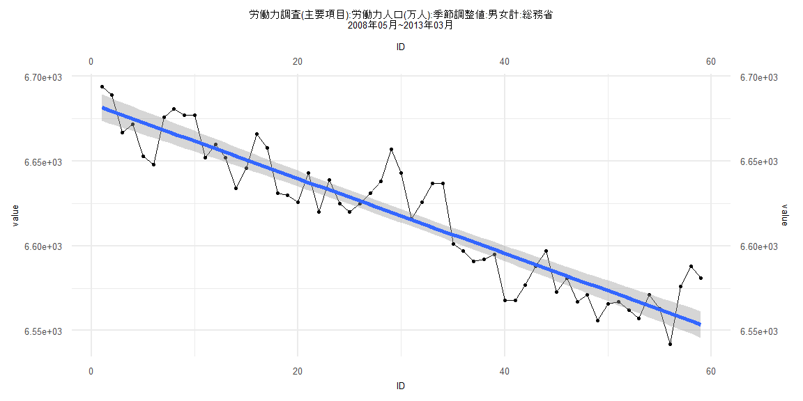
Call:
lm(formula = value ~ ID)

Residuals:
    Min      1Q  Median      3Q     Max
-27.564 -10.724  -3.052  10.960  37.148

Coefficients:
             Estimate Std. Error t value            Pr(>|t|)
(Intercept) 6683.8843     4.0046 1669.04 <0.0000000000000002 ***
ID            -2.2080     0.1161  -19.02 <0.0000000000000002 ***
---
Signif. codes:  0 '***' 0.001 '**' 0.01 '*' 0.05 '.' 0.1 ' ' 1

Residual standard error: 15.18 on 57 degrees of freedom
Multiple R-squared:  0.8639,    Adjusted R-squared:  0.8615
F-statistic: 361.8 on 1 and 57 DF,  p-value: < 0.00000000000000022


    Two-sample Kolmogorov-Smirnov test

data:  lm_residuals and rnorm(n = length(lm_residuals), mean = 0, sd = sd(lm_residuals))
D = 0.10169, p-value = 0.9239
alternative hypothesis: two-sided


    Durbin-Watson test

data:  value ~ ID
DW = 0.96055, p-value = 0.000003776
alternative hypothesis: true autocorrelation is greater than 0


    studentized Breusch-Pagan test

data:  value ~ ID
BP = 1.3358, df = 1, p-value = 0.2478


    Box-Ljung test

data:  lm_residuals
X-squared = 14.621, df = 1, p-value = 0.0001315
Call:
lm(formula = value ~ ID)

Residuals:
    Min      1Q  Median      3Q     Max
-69.668 -26.404   1.447  23.912  67.090

Coefficients:
             Estimate Std. Error t value            Pr(>|t|)
(Intercept) 6532.5589     7.4771  873.68 <0.0000000000000002 ***
ID             4.2939     0.1624   26.44 <0.0000000000000002 ***
---
Signif. codes:  0 '***' 0.001 '**' 0.01 '*' 0.05 '.' 0.1 ' ' 1

Residual standard error: 32.91 on 77 degrees of freedom
Multiple R-squared:  0.9008,    Adjusted R-squared:  0.8995
F-statistic: 699.2 on 1 and 77 DF,  p-value: < 0.00000000000000022


    Two-sample Kolmogorov-Smirnov test

data:  lm_residuals and rnorm(n = length(lm_residuals), mean = 0, sd = sd(lm_residuals))
D = 0.13924, p-value = 0.4302
alternative hypothesis: two-sided


    Durbin-Watson test

data:  value ~ ID
DW = 0.3169, p-value < 0.00000000000000022
alternative hypothesis: true autocorrelation is greater than 0


    studentized Breusch-Pagan test

data:  value ~ ID
BP = 0.0058528, df = 1, p-value = 0.939


    Box-Ljung test

data:  lm_residuals
X-squared = 52.872, df = 1, p-value = 0.000000000000356