日次経済金融指標の計量分析
- 日経平均株価vs東京市場ドル円レート、ダウ平均株価vs日経平均株価、空売り比率vs日経平均株価、ドル円レートvs日経平均株価(月中平均、ベイズ推定)、トランプ大統領の就任前後における日経平均前営業日比ボラティリティの比較 -
アセット・マネジメント・コンサルティング株式会社 https://am-consulting.co.jp
更新日時:2019-12-25 14:06:00
Analysis
日経平均株価と東京市場ドル円レート(Source:日本銀行,日本経済新聞社) ダウ平均株価と日経平均株価(Source:Yahoo Finance,FRED,日本経済新聞社) 空売り比率と日経平均株価(Source:日本取引所グループ、日本経済新聞社) ドル円レートと日経平均株価:ベイズ推定:線形回帰モデル トランプ大統領の就任前後における日経平均前営業日比ボラティリティの比較
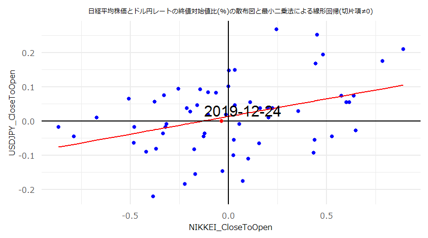
日経平均株価と東京市場ドル円レート(Source:日本銀行,日本経済新聞社)
[1] "USDJPY"
         Date   Open   High    Low  Close Center  Index CloseToOpen HighToLow     MA25 DeviationRate Close:Diff(lag=1) Close:Ratio(lag=1)
56 2019-12-04 108.68 108.67 108.43 108.48 108.55 104.80      -0.184     0.221 108.8936         -0.38             -0.62             -0.568
57 2019-12-05 108.84 108.93 108.78 108.89 108.86 104.78       0.046     0.138 108.8948          0.00              0.41              0.378
58 2019-12-06 108.73 108.78 108.66 108.67 108.78 104.94      -0.055     0.110 108.8972         -0.21             -0.22             -0.202
59 2019-12-09 108.64 108.66 108.55 108.57 108.58 104.98      -0.064     0.101 108.9216         -0.32             -0.10             -0.092
60 2019-12-10 108.59 108.66 108.57 108.63 108.64 104.75       0.037     0.083 108.9152         -0.26              0.06              0.055
61 2019-12-11 108.78 108.86 108.67 108.73 108.74 104.82      -0.046     0.175 108.9052         -0.16              0.10              0.092
62 2019-12-12 108.56 108.65 108.46 108.65 108.58 103.63       0.083     0.175 108.8928         -0.22             -0.08             -0.074
63 2019-12-13 109.40 109.66 108.84 109.63 109.50 103.59       0.210     0.753 108.9064          0.66              0.98              0.902
64 2019-12-16 109.39 109.44 109.30 109.41 109.39 103.35       0.018     0.128 108.9244          0.45             -0.22             -0.201
65 2019-12-17 109.58 109.62 109.49 109.60 109.54 103.47       0.018     0.119 108.9388          0.61              0.19              0.174
66 2019-12-18 109.53 109.57 109.42 109.44 109.44 103.47      -0.082     0.137 108.9536          0.45             -0.16             -0.146
67 2019-12-19 109.55 109.72 109.55 109.58 109.58 103.62       0.027     0.155 108.9868          0.54              0.14              0.128
68 2019-12-20 109.39 109.40 109.26 109.37 109.39 103.61      -0.018     0.128 109.0192          0.32             -0.21             -0.192
69 2019-12-23 109.50 109.54 109.37 109.40 109.42 103.69      -0.091     0.155 109.0384          0.33              0.03              0.027
70 2019-12-24 109.40 109.45 109.37 109.40 109.40     NA       0.000     0.073 109.0676          0.30              0.00              0.000
[1] "NIKKEI"
Date Open High Low Close CloseToOpen HighToLow MA25 DeviationRate Close:Diff(lag=1) Close:Ratio(lag=1)
56 2019-12-04 23186.74 23203.77 23044.78 23135.23 -0.222 0.690 23255.06 -0.52 -244.58 -1.046
57 2019-12-05 23292.70 23363.44 23259.82 23300.09 0.032 0.445 23273.34 0.11 164.86 0.713
58 2019-12-06 23347.67 23412.48 23338.40 23354.40 0.029 0.317 23290.43 0.27 54.31 0.233
59 2019-12-09 23544.31 23544.31 23360.01 23430.70 -0.483 0.789 23313.63 0.50 76.30 0.327
60 2019-12-10 23372.39 23449.47 23336.93 23410.19 0.162 0.482 23319.96 0.39 -20.51 -0.088
61 2019-12-11 23421.14 23438.43 23333.63 23391.86 -0.125 0.449 23323.48 0.29 -18.33 -0.078
62 2019-12-12 23449.28 23468.15 23360.43 23424.81 -0.104 0.461 23327.26 0.42 32.95 0.141
63 2019-12-13 23810.56 24050.04 23775.73 24023.10 0.893 1.154 23352.51 2.87 598.29 2.554
64 2019-12-16 23955.20 24036.30 23950.05 23952.35 -0.012 0.360 23377.33 2.46 -70.75 -0.295
65 2019-12-17 24091.12 24091.12 23996.51 24066.12 -0.104 0.394 23399.17 2.85 113.77 0.475
66 2019-12-18 24023.27 24046.09 23919.36 23934.43 -0.370 0.530 23423.75 2.18 -131.69 -0.547
67 2019-12-19 23911.46 23945.53 23835.29 23864.85 -0.195 0.463 23452.69 1.76 -69.58 -0.291
68 2019-12-20 23893.45 23908.77 23746.63 23816.63 -0.322 0.683 23473.22 1.46 -48.22 -0.202
69 2019-12-23 23921.29 23923.09 23810.82 23821.11 -0.419 0.472 23489.39 1.41 4.48 0.019
70 2019-12-24 23839.18 23853.56 23796.35 23830.58 -0.036 0.240 23510.91 1.36 9.47 0.040単位根検定・共和分検定
- CADFtest {CADFtest}
- ca.po {urca}
$USDJPY_CloseToOpen

    ADF test

data:  x
ADF(0) = -8.9544, p-value = 0.00000000251
alternative hypothesis: true delta is less than 0
sample estimates:
    delta
-1.144612


$NIKKEI_CloseToOpen

    ADF test

data:  x
ADF(1) = -7.2235, p-value = 0.0000004772
alternative hypothesis: true delta is less than 0
sample estimates:
    delta
-1.386642
########################################
# Phillips and Ouliaris Unit Root Test #
########################################

Test of type Pu
detrending of series none


Call:
lm(formula = z[, 1] ~ z[, -1] - 1)

Residuals:
     Min       1Q   Median       3Q      Max
-0.18271 -0.04444  0.01570  0.08951  0.24238

Coefficients:
        Estimate Std. Error t value Pr(>|t|)
z[, -1]  0.10416    0.03209   3.246  0.00193 **
---
Signif. codes:  0 '***' 0.001 '**' 0.01 '*' 0.05 '.' 0.1 ' ' 1

Residual standard error: 0.09605 on 59 degrees of freedom
Multiple R-squared:  0.1515,    Adjusted R-squared:  0.1372
F-statistic: 10.54 on 1 and 59 DF,  p-value: 0.00193


Value of test-statistic is: 68.6696

Critical values of Pu are:
                  10pct    5pct    1pct
critical values 20.3933 25.9711 38.3413
最小二乗法
- lm {stats}
- dwtest {lmtest}
- ks.test {stats}
- confint {stats}
- Box.test {stats}
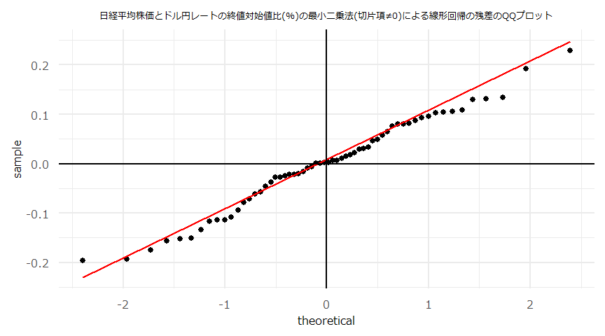
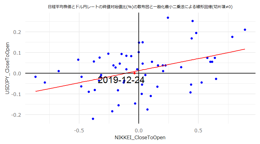
- 切片項\(\neq0\)
MODEL INFO:
Observations: 60
Dependent Variable: USDJPY_CloseToOpen
Type: OLS linear regression

MODEL FIT:
F(1,58) = 10.31, p = 0.00
R2 = 0.15
Adj. R2 = 0.14

Standard errors: OLS
---------------------------------------------------------------
                           Est.    2.5%   97.5%   t val.      p
------------------------ ------ ------- ------- -------- ------
(Intercept)                0.01   -0.01    0.04     1.06   0.29
NIKKEI_CloseToOpen         0.10    0.04    0.17     3.21   0.00
---------------------------------------------------------------
    Durbin-Watson test

data:  OLS_Model
DW = 2.4114, p-value = 0.9467
alternative hypothesis: true autocorrelation is greater than 0
    One-sample Kolmogorov-Smirnov test

data:  ResidualsOLS
D = 0.084468, p-value = 0.7534
alternative hypothesis: two-sided
2.5 % 97.5 %
(Intercept) -0.01163023 0.03798747
NIKKEI_CloseToOpen 0.03878814 0.16717655
Box-Ljung test
data: ResidualsOLS
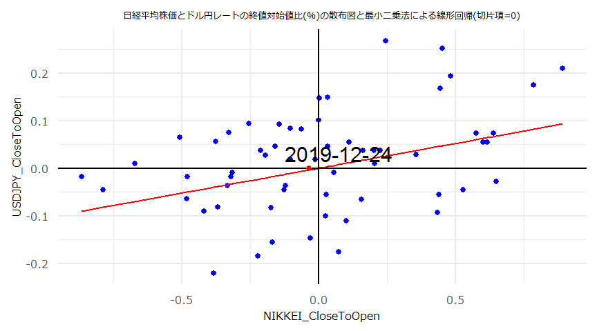
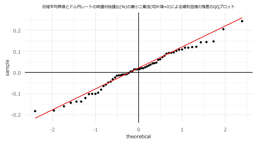
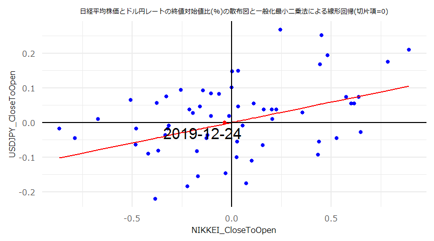
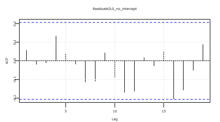
X-squared = 14.481, df = 10, p-value = 0.1522- 切片項\(=0\)
MODEL INFO:
Observations: 60
Dependent Variable: USDJPY_CloseToOpen
Type: OLS linear regression

MODEL FIT:
F(1,59) = 10.54, p = 0.00
R2 = 0.15
Adj. R2 = 0.14

Standard errors: OLS
--------------------------------------------------------------
                           Est.   2.5%   97.5%   t val.      p
------------------------ ------ ------ ------- -------- ------
NIKKEI_CloseToOpen         0.10   0.04    0.17     3.25   0.00
--------------------------------------------------------------
    Durbin-Watson test

data:  OLS_Model_no_intercept
DW = 2.3652, p-value = 0.9408
alternative hypothesis: true autocorrelation is greater than 0
    One-sample Kolmogorov-Smirnov test

data:  ResidualsOLS_no_intercept
D = 0.13805, p-value = 0.1849
alternative hypothesis: two-sided
2.5 % 97.5 %
NIKKEI_CloseToOpen 0.03995344 0.1683613
    Box-Ljung test

data:  ResidualsOLS_no_intercept
X-squared = 14.587, df = 10, p-value = 0.1479
一般化最小二乗法
- gls {nlme}
- corARMA {nlme}
- ks.test {stats}
- confint {stats}
- Box.test {stats}
- 残差の系列相関の有無に拘わらず一般化最小二乗法による回帰係数を求めています。
- 最小二乗法の残差に系列相関が見られない場合、ここではAR(\(p=0,q=0\))の結果(AIC最小)が表示されます。
- http://user.keio.ac.jp/~nagakura/zemi/GLS.pdf
- http://tokyox.matrix.jp/wiki/index.php?%E4%B8%80%E8%88%AC%E5%8C%96%E6%9C%80%E5%B0%8F%E4%BA%8C%E4%B9%97%E6%B3%95
- 切片項\(\neq0\)
Generalized least squares fit by REML
  Model: USDJPY_CloseToOpen ~ NIKKEI_CloseToOpen
  Data: USDJPY_NIKKEI
       AIC       BIC  logLik
  -96.3286 -86.02638 53.1643

Correlation Structure: ARMA(1,1)
 Formula: ~1
 Parameter estimate(s):
      Phi1     Theta1
-0.8426918  0.6615541

Coefficients:
                        Value  Std.Error  t-value p-value
(Intercept)        0.01243702 0.01064200 1.168674  0.2473
NIKKEI_CloseToOpen 0.11609381 0.02898921 4.004726  0.0002

 Correlation:
                   (Intr)
NIKKEI_CloseToOpen -0.037

Standardized residuals:
        Min          Q1         Med          Q3         Max
-2.03575806 -0.54324309  0.03505838  0.78076549  2.35744431

Residual standard error: 0.09629237
Degrees of freedom: 60 total; 58 residual
    One-sample Kolmogorov-Smirnov test

data:  ResidualsGLS
D = 0.080139, p-value = 0.8063
alternative hypothesis: two-sided
2.5 % 97.5 %
(Intercept) -0.008420907 0.03329496
NIKKEI_CloseToOpen 0.059276016 0.17291161
    Box-Ljung test

data:  ResidualsGLS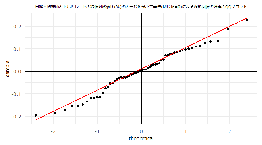
X-squared = 15.627, df = 10, p-value = 0.1108- 切片項\(=0\)
Generalized least squares fit by REML
  Model: USDJPY_CloseToOpen ~ NIKKEI_CloseToOpen - 1
  Data: USDJPY_NIKKEI
        AIC       BIC  logLik
  -104.2126 -95.90245 56.1063

Correlation Structure: ARMA(1,1)
 Formula: ~1
 Parameter estimate(s):
      Phi1     Theta1
-0.8464688  0.6655166

Coefficients:
                       Value Std.Error  t-value p-value
NIKKEI_CloseToOpen 0.1174511 0.0290519 4.042804  0.0002

Standardized residuals:
       Min         Q1        Med         Q3        Max
-1.8998827 -0.4070335  0.1609874  0.9135233  2.4730353

Residual standard error: 0.09668565
Degrees of freedom: 60 total; 59 residual
    One-sample Kolmogorov-Smirnov test

data:  ResidualsGLS_no_intercept
D = 0.12728, p-value = 0.2624
alternative hypothesis: two-sided
2.5 % 97.5 %
NIKKEI_CloseToOpen 0.06051046 0.1743918
Box-Ljung test
data: ResidualsGLS_no_intercept
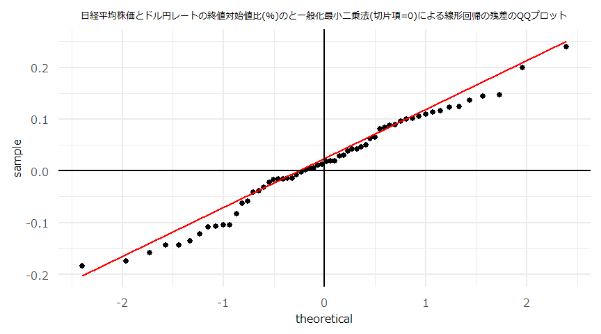
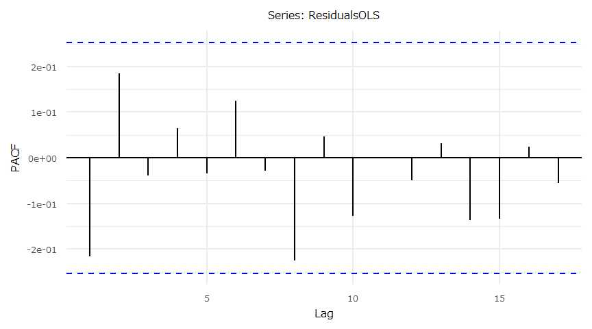
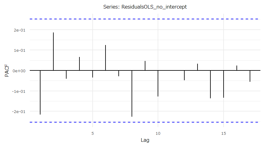
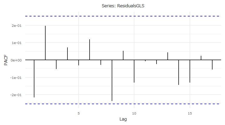
X-squared = 15.739, df = 10, p-value = 0.1073散布図・QQプロット・残差の時系列推移
- (注意)線形回帰の傾き(\(a\))、切片(\(b\))それぞれの検定統計量、p値に関わらず\(y=ax+b\)とした回帰直線やその残差を散布図、QQプロット等にプロットしています。
- 散布図とQQプロット
- 残差の自己相関(ACF)
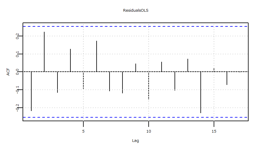
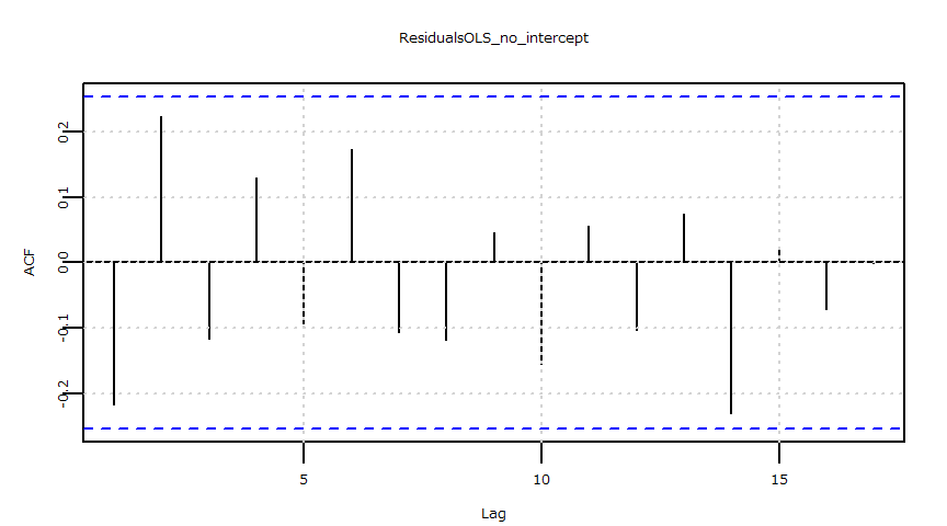
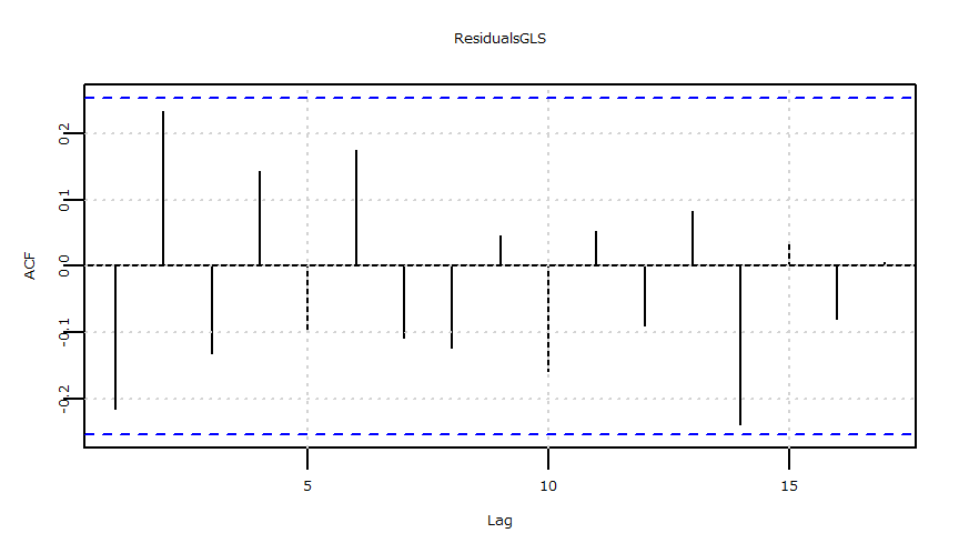

- 残差の自己相関(PACF)

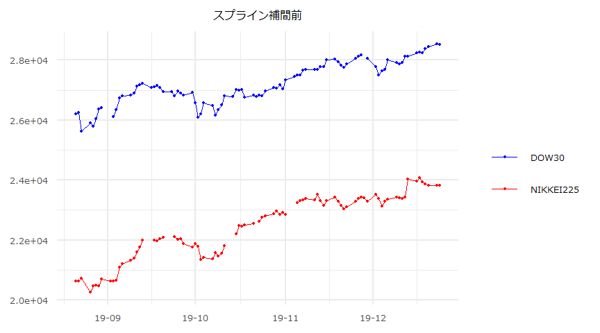
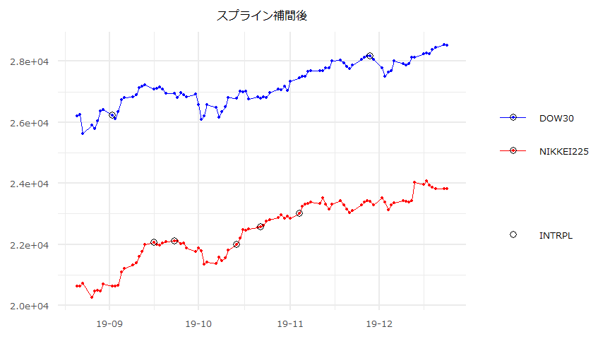
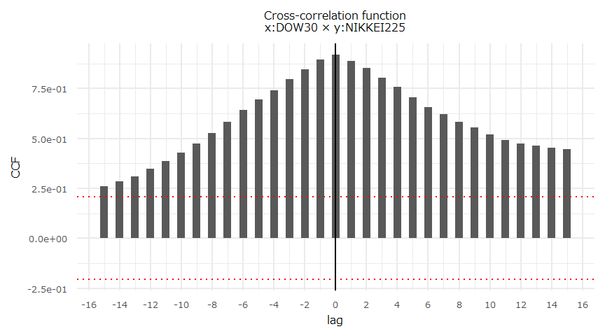
ダウ平均株価と日経平均株価(Source:Yahoo Finance,FRED,日本経済新聞社)
時系列チャート
- Source:
- (注意) 欠損値(休場日)は原系列にスプライン補間を掛けた上で前日比を算出している。
- 対象期間:2019-08-21~2019-12-24
- サンプルサイズ:n=90
単位根検定・共和分検定
- CADFtest {CADFtest}
- ca.po {urca}
単位根検定
$DOW30

    ADF test

data:  x
ADF(0) = -2.591, p-value = 0.2855
alternative hypothesis: true delta is less than 0
sample estimates:
     delta
-0.1330281


$NIKKEI225

    ADF test

data:  x
ADF(0) = -2.0945, p-value = 0.5413
alternative hypothesis: true delta is less than 0
sample estimates:
     delta
-0.1023453


$DOW30_Change

    ADF test

data:  x
ADF(2) = -7.2466, p-value = 0.00000009042
alternative hypothesis: true delta is less than 0
sample estimates:
    delta
-1.282188


$NIKKEI225_Change

    ADF test

data:  x
ADF(0) = -9.1982, p-value = 0.00000000005683
alternative hypothesis: true delta is less than 0
sample estimates:
    delta
-1.003339
共和分検定
[1] "DOW30 × NIKKEI225"
########################################
# Phillips and Ouliaris Unit Root Test #
########################################
Test of type Pu
detrending of series none
Call:
lm(formula = z[, 1] ~ z[, -1] - 1)
Residuals:
Min 1Q Median 3Q Max
-967.2 -484.4 -195.3 445.3 1575.1
Coefficients:
Estimate Std. Error t value Pr(>|t|)
z[, -1] 1.211440 0.003134 386.5 <0.0000000000000002 ***
---
Signif. codes: 0 '***' 0.001 '**' 0.01 '*' 0.05 '.' 0.1 ' ' 1
Residual standard error: 667.9 on 89 degrees of freedom
Multiple R-squared: 0.9994, Adjusted R-squared: 0.9994
F-statistic: 1.494e+05 on 1 and 89 DF, p-value: < 0.00000000000000022
Value of test-statistic is: 3.9619
Critical values of Pu are:
10pct 5pct 1pct
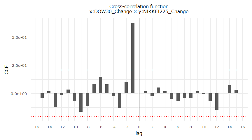
critical values 20.3933 25.9711 38.3413相互相関関数
- ggCcf {forecast}
ベクトル自己回帰モデル
- VARselect {vars}
- VAR {vars}
VAR Estimation Results:
=========================
Endogenous variables: DOW30, NIKKEI225
Deterministic variables: const
Sample size: 89
Log Likelihood: -1151.782
Roots of the characteristic polynomial:
0.9886 0.7546
Call:
VAR(y = obj, p = selected_lag, type = "const")


Estimation results for equation DOW30:
======================================
DOW30 = DOW30.l1 + NIKKEI225.l1 + const

               Estimate Std. Error t value            Pr(>|t|)
DOW30.l1        0.88230    0.06605  13.358 <0.0000000000000002 ***
NIKKEI225.l1    0.07046    0.04500   1.566               0.121
const        1647.32153  957.73430   1.720               0.089 .
---
Signif. codes:  0 '***' 0.001 '**' 0.01 '*' 0.05 '.' 0.1 ' ' 1


Residual standard error: 173.7 on 86 degrees of freedom
Multiple R-Squared: 0.942,  Adjusted R-squared: 0.9406
F-statistic:   698 on 2 and 86 DF,  p-value: < 0.00000000000000022


Estimation results for equation NIKKEI225:
==========================================
NIKKEI225 = DOW30.l1 + NIKKEI225.l1 + const

                Estimate  Std. Error t value             Pr(>|t|)
DOW30.l1         0.19275     0.05558   3.468             0.000821 ***
NIKKEI225.l1     0.86088     0.03786  22.737 < 0.0000000000000002 ***
const        -2086.44362   805.89249  -2.589             0.011302 *
---
Signif. codes:  0 '***' 0.001 '**' 0.01 '*' 0.05 '.' 0.1 ' ' 1


Residual standard error: 146.1 on 86 degrees of freedom
Multiple R-Squared: 0.9803, Adjusted R-squared: 0.9799
F-statistic:  2145 on 2 and 86 DF,  p-value: < 0.00000000000000022


Covariance matrix of residuals:
          DOW30 NIKKEI225
DOW30     30165      2271
NIKKEI225  2271     21358

Correlation matrix of residuals:
            DOW30 NIKKEI225
DOW30     1.00000   0.08945
NIKKEI225 0.08945   1.00000
VAR Estimation Results:
=========================
Endogenous variables: DOW30_Change, NIKKEI225_Change
Deterministic variables: const
Sample size: 89
Log Likelihood: -159.944
Roots of the characteristic polynomial:
0.1094 0.09431
Call:
VAR(y = obj, p = selected_lag, type = "const")
Estimation results for equation DOW30_Change:
=============================================
DOW30_Change = DOW30_Change.l1 + NIKKEI225_Change.l1 + const
Estimate Std. Error t value Pr(>|t|)
DOW30_Change.l1 0.01659 0.10692 0.155 0.877
NIKKEI225_Change.l1 0.01535 0.10015 0.153 0.879
const 0.09291 0.07289 1.275 0.206
Residual standard error: 0.6615 on 86 degrees of freedom
Multiple R-Squared: 0.0005554, Adjusted R-squared: -0.02269
F-statistic: 0.0239 on 2 and 86 DF, p-value: 0.9764
Estimation results for equation NIKKEI225_Change:
=================================================
NIKKEI225_Change = DOW30_Change.l1 + NIKKEI225_Change.l1 + const
Estimate Std. Error t value Pr(>|t|)
DOW30_Change.l1 0.670169 0.089309 7.504 0.0000000000527 ***
NIKKEI225_Change.l1 -0.001546 0.083650 -0.018 0.985
const 0.092429 0.060883 1.518 0.133
---
Signif. codes: 0 '***' 0.001 '**' 0.01 '*' 0.05 '.' 0.1 ' ' 1
Residual standard error: 0.5525 on 86 degrees of freedom
Multiple R-Squared: 0.3957, Adjusted R-squared: 0.3816
F-statistic: 28.15 on 2 and 86 DF, p-value: 0.000000000393
Covariance matrix of residuals:
DOW30_Change NIKKEI225_Change
DOW30_Change 0.437596 0.001839
NIKKEI225_Change 0.001839 0.305302
Correlation matrix of residuals:
DOW30_Change NIKKEI225_Change
DOW30_Change 1.00000 0.00503
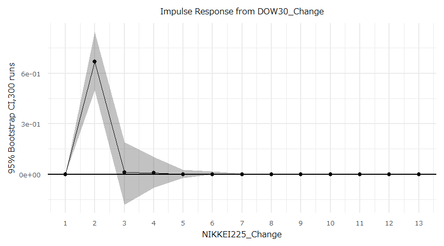
NIKKEI225_Change 0.00503 1.00000グレンジャー因果
- causality {vars}
Dow → Nikkei
Granger causality H0: DOW30_Change do not Granger-cause NIKKEI225_Change
data: VAR object var_result
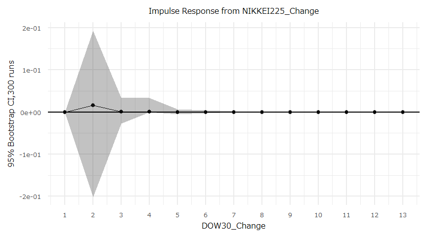
F-Test = 56.309, df1 = 1, df2 = 172, p-value = 0.000000000003182Nikkei → Dow
Granger causality H0: NIKKEI225_Change do not Granger-cause DOW30_Change
data: VAR object var_result
F-Test = 0.023496, df1 = 1, df2 = 172, p-value = 0.8784インパルス応答
- irf {vars}
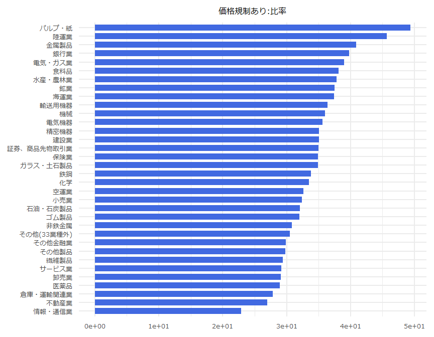
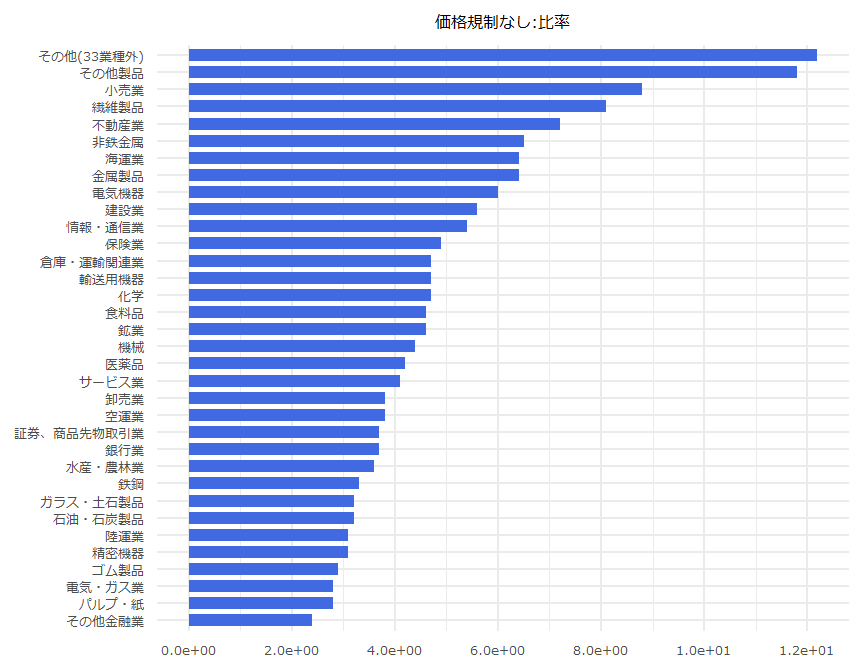
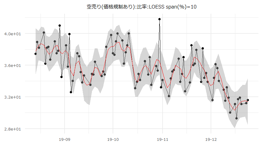
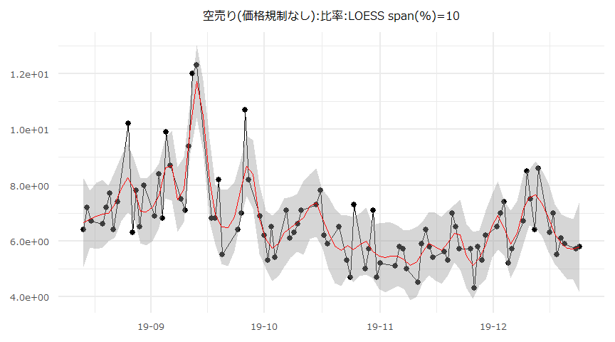
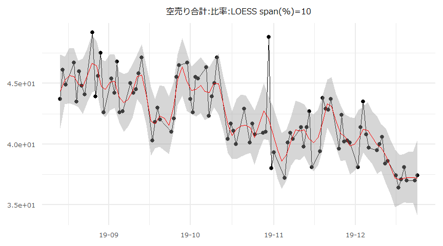
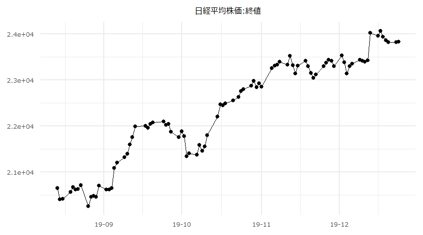
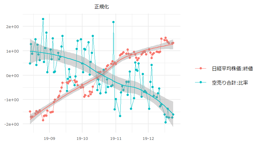
空売り比率と日経平均株価(Source:日本取引所グループ、日本経済新聞社)
業種別空売り集計
- 2019年12月24日
- 「空売り合計:比率」は100から「実注文:比率」を減じた数値としています。
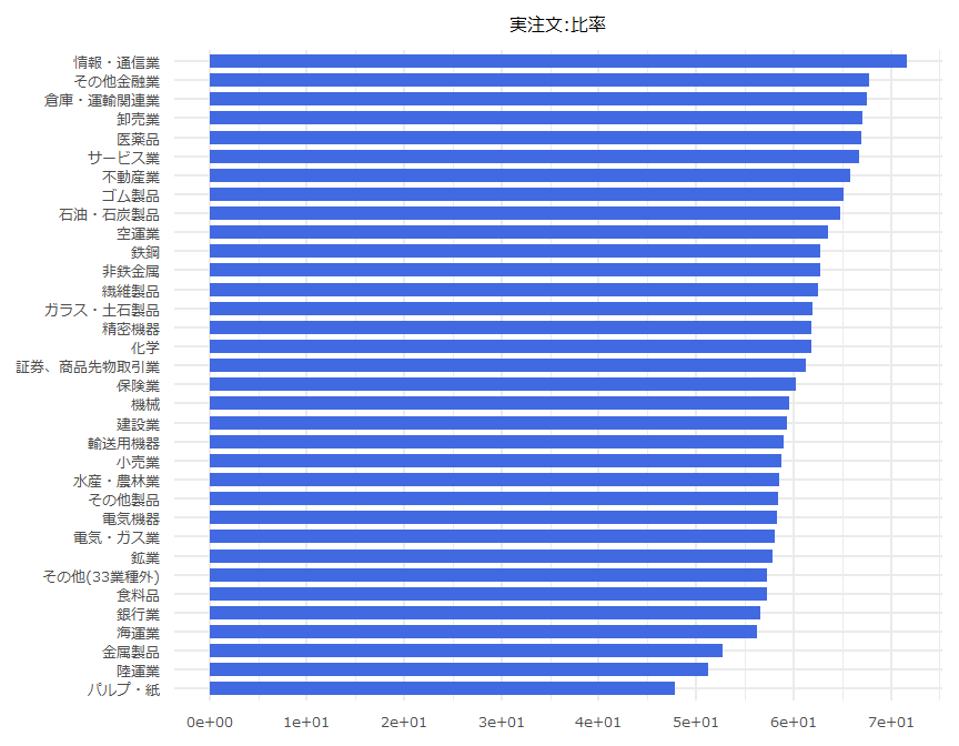
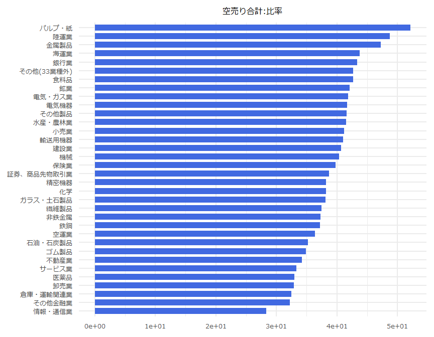
| N | 業種名 | 空売り合計:比率 |
|---|---|---|
| 1 | 水産・農林業 | 41.5 |
| 2 | 鉱業 | 42.1 |
| 3 | 建設業 | 40.7 |
| 4 | 食料品 | 42.7 |
| 5 | 繊維製品 | 37.5 |
| 6 | パルプ・紙 | 52.2 |
| 7 | 化学 | 38.2 |
| 8 | 医薬品 | 33 |
| 9 | 石油・石炭製品 | 35.2 |
| 10 | ゴム製品 | 34.9 |
| 11 | ガラス・土石製品 | 38.1 |
| 12 | 鉄鋼 | 37.2 |
| 13 | 非鉄金属 | 37.3 |
| 14 | 金属製品 | 47.3 |
| 15 | 機械 | 40.4 |
| 16 | 電気機器 | 41.7 |
| 17 | 輸送用機器 | 41 |
| 18 | 精密機器 | 38.2 |
| 19 | その他製品 | 41.6 |
| 20 | 電気・ガス業 | 41.9 |
| 21 | 陸運業 | 48.8 |
| 22 | 海運業 | 43.8 |
| 23 | 空運業 | 36.4 |
| 24 | 倉庫・運輸関連業 | 32.5 |
| 25 | 情報・通信業 | 28.3 |
| 26 | 卸売業 | 32.9 |
| 27 | 小売業 | 41.2 |
| 28 | 銀行業 | 43.4 |
| 29 | 証券、商品先物取引業 | 38.7 |
| 30 | 保険業 | 39.8 |
| 31 | その他金融業 | 32.2 |
| 32 | 不動産業 | 34.2 |
| 33 | サービス業 | 33.3 |
| 34 | その他(33業種外) | 42.7 |
空売り比率の時系列推移
- 2019-08-14 ~ 2019-12-24

| Date | 12-24 | 12-23 | 12-20 | 12-19 | 12-18 | 12-17 | 12-16 | 12-13 |
|---|---|---|---|---|---|---|---|---|
| 実注文:比率 | 62.6 | 63 | 63 | 61.9 | 62.9 | 63.6 | 62.6 | 61.4 |
| 空売り(価格規制あり):比率 | 31.6 | 31.2 | 31.1 | 31.9 | 31.7 | 29.3 | 31.1 | 30 |
| 空売り(価格規制なし):比率 | 5.8 | 5.7 | 5.9 | 6.1 | 5.5 | 7 | 6.3 | 8.6 |
| 空売り合計:比率 | 37.4 | 37 | 37 | 38.1 | 37.1 | 36.4 | 37.4 | 38.6 |
日経平均株価と空売り比率
時系列推移
- 対象期間:2019-08-14 ~ 2019-12-24
単位根検定/共和分検定
- CADFtest {CADFtest}
- ca.po {urca}
- 各系列の“_change“は前営業日との差。
- 対象期間: 2019-08-14 ~ 2019-12-24,90days
### 単位根検定 ###

$NIKKEI225.close

    ADF test

data:  x
ADF(0) = -2.1666, p-value = 0.5017
alternative hypothesis: true delta is less than 0
sample estimates:
     delta
-0.1102726


$ShortSalerRatio

    ADF test

data:  x
ADF(0) = -7.9666, p-value = 0.000000005333
alternative hypothesis: true delta is less than 0
sample estimates:
     delta
-0.8607999


$NIKKEI225.close_change

    ADF test

data:  x
ADF(0) = -9.1907, p-value = 0.00000000005833
alternative hypothesis: true delta is less than 0
sample estimates:
    delta
-1.002416


$ShortSalerRatio_change

    ADF test

data:  x
ADF(2) = -8.8201, p-value = 0.0000000002165
alternative hypothesis: true delta is less than 0
sample estimates:
    delta
-2.348904
### 共和分検定 ###
########################################
# Phillips and Ouliaris Unit Root Test #
########################################
Test of type Pu
detrending of series none
Call:
lm(formula = z[, 1] ~ z[, -1] - 1)
Residuals:
Min 1Q Median 3Q Max
-5551.2 -2270.9 586.3 2250.0 4969.2
Coefficients:
Estimate Std. Error t value Pr(>|t|)
z[, -1] 524.640 6.377 82.28 <0.0000000000000002 ***
---
Signif. codes: 0 '***' 0.001 '**' 0.01 '*' 0.05 '.' 0.1 ' ' 1
Residual standard error: 2562 on 89 degrees of freedom
Multiple R-squared: 0.987, Adjusted R-squared: 0.9869
F-statistic: 6769 on 1 and 89 DF, p-value: < 0.00000000000000022
Value of test-statistic is: 0.2996
Critical values of Pu are:
10pct 5pct 1pct
critical values 20.3933 25.9711 38.3413最小二乗法
- lm {stats}
- dwtest {lmtest}
- ks.test {stats}
- confint {stats}
- Box.test {stats}
- Ljung-Box 検定のラグは15としている。
- 対象期間: 2019-08-14 ~ 2019-12-24,90days
- 切片項\(\neq0\)
Call:
lm(formula = NIKKEI225.close_change ~ ShortSalerRatio_change,
    data = datadf)

Residuals:
    Min      1Q  Median      3Q     Max
-387.74  -70.73  -11.15   73.78  569.85

Coefficients:
                       Estimate Std. Error t value   Pr(>|t|)
(Intercept)              34.182     15.347   2.227     0.0285 *
ShortSalerRatio_change  -28.729      5.653  -5.082 0.00000208 ***
---
Signif. codes:  0 '***' 0.001 '**' 0.01 '*' 0.05 '.' 0.1 ' ' 1

Residual standard error: 145.5 on 88 degrees of freedom
Multiple R-squared:  0.2269,    Adjusted R-squared:  0.2181
F-statistic: 25.82 on 1 and 88 DF,  p-value: 0.000002082
    Durbin-Watson test

data:  OLS_Model
DW = 1.88, p-value = 0.3013
alternative hypothesis: true autocorrelation is greater than 0
    One-sample Kolmogorov-Smirnov test

data:  ResidualsOLS
D = 0.079749, p-value = 0.588
alternative hypothesis: two-sided
2.5 % 97.5 %
(Intercept) 3.682693 64.68076
ShortSalerRatio_change -39.964450 -17.49417
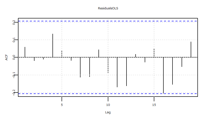
    Box-Ljung test

data:  ResidualsOLS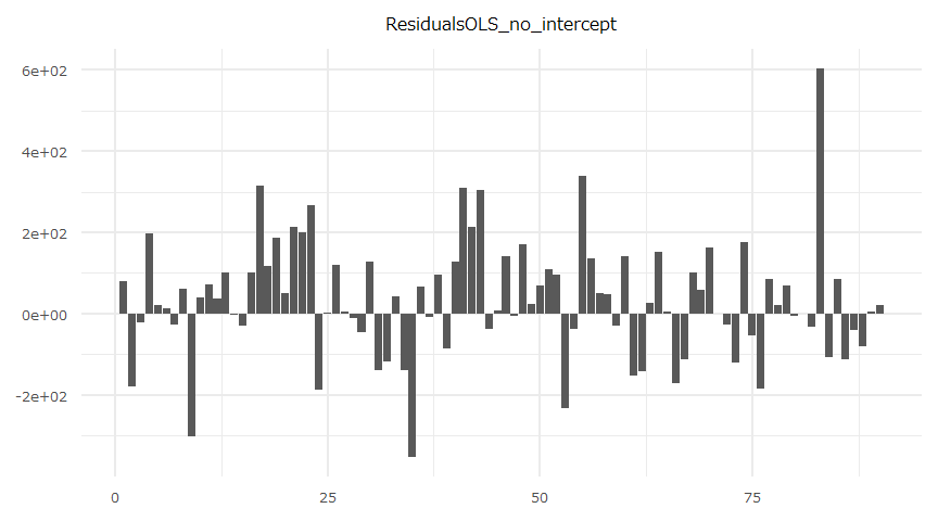
X-squared = 11.949, df = 15, p-value = 0.6829- 切片項\(=0\)
Call:
lm(formula = NIKKEI225.close_change ~ ShortSalerRatio_change -
    1, data = datadf)

Residuals:
    Min      1Q  Median      3Q     Max
-352.00  -36.53   22.49  107.50  604.14

Coefficients:
                       Estimate Std. Error t value   Pr(>|t|)
ShortSalerRatio_change  -29.265      5.773   -5.07 0.00000215 ***
---
Signif. codes:  0 '***' 0.001 '**' 0.01 '*' 0.05 '.' 0.1 ' ' 1

Residual standard error: 148.7 on 89 degrees of freedom
Multiple R-squared:  0.2241,    Adjusted R-squared:  0.2154
F-statistic:  25.7 on 1 and 89 DF,  p-value: 0.000002151
    Durbin-Watson test

data:  OLS_Model_no_intercept
DW = 1.7822, p-value = 0.1892
alternative hypothesis: true autocorrelation is greater than 0
    One-sample Kolmogorov-Smirnov test

data:  ResidualsOLS_no_intercept
D = 0.16801, p-value = 0.01088
alternative hypothesis: two-sided
2.5 % 97.5 %
ShortSalerRatio_change -40.73552 -17.79511
    Box-Ljung test

data:  ResidualsOLS_no_intercept
X-squared = 11.895, df = 15, p-value = 0.687
一般化最小二乗法
- gls {nlme}
- corARMA {nlme}
- ks.test {stats}
- confint {stats}
- Box.test {stats}
- 残差の系列相関の有無に拘わらず一般化最小二乗法による回帰係数を求めています。
- 最小二乗法の残差に系列相関が見られない場合、ここではAR(p=0,q=0)の結果(AIC最小)が表示されます。
- http://user.keio.ac.jp/~nagakura/zemi/GLS.pdf
- http://tokyox.matrix.jp/wiki/index.php?%E4%B8%80%E8%88%AC%E5%8C%96%E6%9C%80%E5%B0%8F%E4%BA%8C%E4%B9%97%E6%B3%95
- Ljung-Box 検定のラグは15としている。
- 切片項\(\neq0\)
Generalized least squares fit by REML
  Model: NIKKEI225.close_change ~ ShortSalerRatio_change
  Data: datadf
       AIC      BIC    logLik
  1143.194 1150.626 -568.5972

Coefficients:
                           Value Std.Error   t-value p-value
(Intercept)             34.18172 15.347047  2.227251  0.0285
ShortSalerRatio_change -28.72931  5.653498 -5.081687  0.0000

 Correlation:
                       (Intr)
ShortSalerRatio_change 0.043

Standardized residuals:
        Min          Q1         Med          Q3         Max
-2.66553684 -0.48624141 -0.07665896  0.50723977  3.91752212

Residual standard error: 145.4629
Degrees of freedom: 90 total; 88 residual
    One-sample Kolmogorov-Smirnov test

data:  ResidualsGLS
D = 0.079749, p-value = 0.588
alternative hypothesis: two-sided
2.5 % 97.5 %
(Intercept) 4.102064 64.26138
ShortSalerRatio_change -39.809963 -17.64866
    Box-Ljung test

data:  ResidualsGLS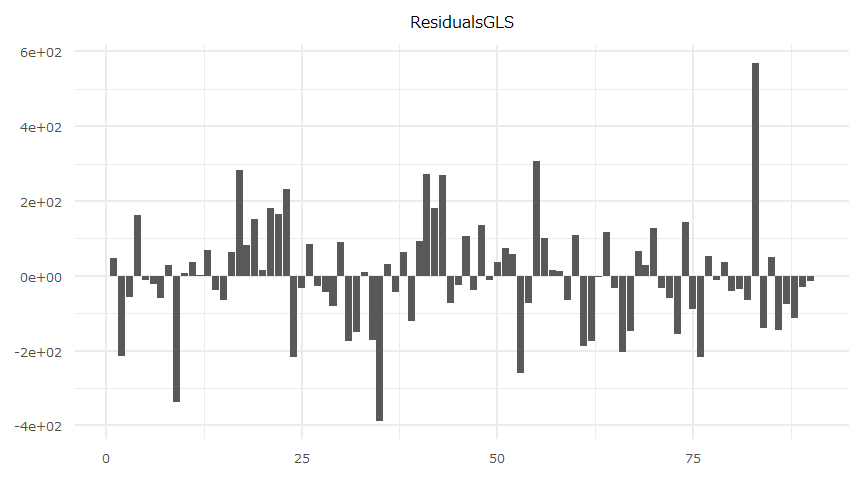
X-squared = 11.949, df = 15, p-value = 0.6829- 切片項\(=0\)
Generalized least squares fit by REML
  Model: NIKKEI225.close_change ~ ShortSalerRatio_change - 1
  Data: datadf
       AIC      BIC    logLik
  1153.369 1158.346 -574.6846

Coefficients:
                           Value Std.Error   t-value p-value
ShortSalerRatio_change -29.26532  5.772687 -5.069618       0

Standardized residuals:
       Min         Q1        Med         Q3        Max
-2.3677540 -0.2457028  0.1513119  0.7231028  4.0638061

Residual standard error: 148.6643
Degrees of freedom: 90 total; 89 residual
    One-sample Kolmogorov-Smirnov test

data:  ResidualsGLS_no_intercept
D = 0.16801, p-value = 0.01088
alternative hypothesis: two-sided
2.5 % 97.5 %
ShortSalerRatio_change -40.57957 -17.95106
    Box-Ljung test

data:  ResidualsGLS_no_intercept
X-squared = 11.895, df = 15, p-value = 0.687
残差
- 時系列推移
- 自己相関
- 時系列推移


- 自己相関


ドル円レートと日経平均株価:ベイズ推定:線形回帰モデル
\[\rm{NIKKEI}\sim\rm{Normal}(\beta_0 + \beta_1 \cdot \rm{USDJPY},\sigma)\]
# 数値はいずれも前月比(%)
head(df)
Date NIKKEI USDJPY
13 2017-01-01 0.67 -1.05
14 2017-02-01 -0.03 -1.45
15 2017-03-01 0.79 -0.05
16 2017-04-01 -3.12 -2.59
17 2017-05-01 5.29 1.94
18 2017-06-01 1.62 -1.19tail(df) Date NIKKEI USDJPY
43 2019-07-01 2.53 0.15
44 2019-08-01 -4.46 -1.81
45 2019-09-01 4.63 1.06
46 2019-10-01 2.84 0.65
47 2019-11-01 4.87 0.69
48 2019-12-01 1.50 0.26apply(df[, -1], 2, adf.test)$NIKKEI
Augmented Dickey-Fuller Test
data: newX[, i]
Dickey-Fuller = -3.5875, Lag order = 3, p-value = 0.04791
alternative hypothesis: stationary
$USDJPY
Augmented Dickey-Fuller Test
data: newX[, i]
Dickey-Fuller = -4.1669, Lag order = 3, p-value = 0.01457
alternative hypothesis: stationary# 最尤推定
summary(lm(NIKKEI ~ USDJPY), confint = T, ci.width = 0.95)
Call:
lm(formula = NIKKEI ~ USDJPY)

Residuals:
    Min      1Q  Median      3Q     Max
-4.7835 -1.1220  0.2934  1.2350  6.0612

Coefficients:
            Estimate Std. Error t value  Pr(>|t|)
(Intercept)   0.8789     0.4230   2.078    0.0454 *
USDJPY        1.4584     0.2974   4.903 0.0000229 ***
---
Signif. codes:  0 '***' 0.001 '**' 0.01 '*' 0.05 '.' 0.1 ' ' 1

Residual standard error: 2.523 on 34 degrees of freedom
Multiple R-squared:  0.4142,    Adjusted R-squared:  0.397
F-statistic: 24.04 on 1 and 34 DF,  p-value: 0.00002293
Gaussian <- "
data{
int N;
vector[N] NIKKEI;
vector[N] USDJPY;
}
parameters{
real beta0;
real beta1;
real <lower = 0> sigma;
}
model{
for(i in 1:N)
NIKKEI[i] ~ normal(beta0 + beta1*USDJPY[i], sigma);
}
generated quantities{
vector[N] pred_NIKKEI;
real log_lik[N];
for (i in 1:N){
pred_NIKKEI[i] = normal_rng(beta0 + beta1*USDJPY[i], sigma);
log_lik[i] = normal_lpdf(NIKKEI[i] | beta0 + beta1*USDJPY[i], sigma);
}
}
"datalist <- list(N = N, NIKKEI = NIKKEI, USDJPY = USDJPY)
iter <- 1400
warmup <- 400
chains <- 3
fit <- stan(model_code = Gaussian, data = datalist, iter = iter, warmup = warmup, thin = 1, chains = chains)
summary(fit)$summary[c("beta0", "beta1", "sigma"), ] mean se_mean sd 2.5% 25% 50% 75% 97.5% n_eff Rhat
beta0 0.8875346 0.009630047 0.4428774 0.03346326 0.5973444 0.8823194 1.186767 1.786213 2114.999 1.0008931
beta1 1.4635474 0.005635220 0.2999310 0.87680494 1.2622379 1.4641785 1.659193 2.056325 2832.833 0.9997827
sigma 2.6145262 0.006997019 0.3353027 2.03981008 2.3895432 2.5752479 2.804797 3.363150 2296.402 1.0004320traceplot(fit) + theme(axis.text.x = element_text(size = 5), axis.text.y = element_text(size = 5), strip.text.x = element_text(size = 5), legend.title = element_text(size = 5), legend.text = element_text(size = 5))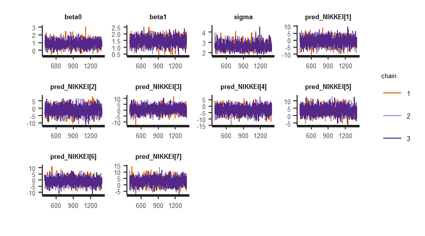
# EAP:事後期待値
df_result <- rstan::extract(fit)$pred_NIKKEI %>% data.frame() %>% gather() %>% dplyr::mutate(id = rep(c(1:N), each = (iter - warmup) * chains)) %>% group_by(id) %>% dplyr::summarize(pred_EAP = mean(value), pred_lower = quantile(value, 0.025), pred_upper = quantile(value, 0.975)) %>% dplyr::ungroup() %>% cbind(data.frame(NIKKEI, USDJPY))
head(df_result) id pred_EAP pred_lower pred_upper NIKKEI USDJPY
1 1 -0.6670891 -5.887419 4.747134 0.67 -1.05
2 2 -1.3311440 -6.746644 4.062978 -0.03 -1.45
3 3 0.8456611 -4.601861 6.233359 0.79 -0.05
4 4 -2.8765245 -8.453013 2.506951 -3.12 -2.59
5 5 3.7032181 -1.472681 9.062403 5.29 1.94
6 6 -0.9205032 -6.276003 4.648296 1.62 -1.19tail(df_result) id pred_EAP pred_lower pred_upper NIKKEI USDJPY
31 31 1.049604 -4.285724 6.165953 2.53 0.15
32 32 -1.777217 -7.089221 3.549118 -4.46 -1.81
33 33 2.382464 -2.890374 7.561279 4.63 1.06
34 34 1.833427 -3.393662 7.165621 2.84 0.65
35 35 1.898318 -3.377486 7.176082 4.87 0.69
36 36 1.217293 -4.193934 6.568841 1.50 0.26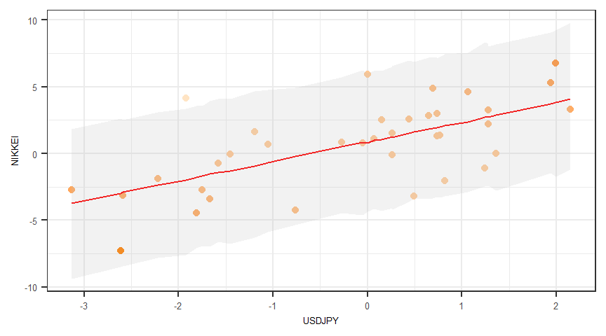
トランプ大統領の就任前後における日経平均前営業日比ボラティリティの比較
- 休日、祝日の補間はとっていない。
- helpより
- 『garchOrder The ARCH (q) and GARCH (p) orders.』
- 『external.regressors A matrix object containing the external regressors to include in the variance equation with as many rows as will be included in the data (which is passed in the fit function).』
- 参照引用Webページ
head(nikkei) Date Nikkei_ChangeRate trump
14882 2009-01-20 -2.313958 0
14883 2009-01-21 -2.035139 0
14884 2009-01-22 1.899606 0
14885 2009-01-23 -3.806506 0
14886 2009-01-26 -0.814822 0
14887 2009-01-27 4.932610 0tail(nikkei) Date Nikkei_ChangeRate trump
17554 2019-12-17 0.47498471 1
17555 2019-12-18 -0.54720080 1
17556 2019-12-19 -0.29071091 1
17557 2019-12-20 -0.20205449 1
17558 2019-12-23 0.01881039 1
17559 2019-12-24 0.03975465 1head(nikkei[as.Date("2017-1-17") <= nikkei$Date, ]) Date Nikkei_ChangeRate trump
16839 2017-01-17 -1.4752891 0
16840 2017-01-18 0.4296908 0
16841 2017-01-19 0.9414445 0
16842 2017-01-20 0.3442698 1
16843 2017-01-23 -1.2900050 1
16844 2017-01-24 -0.5454441 1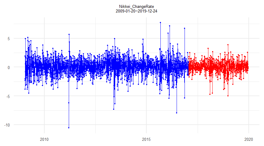
nikkei$trump <- as.numeric(nikkei$trump)datavalue <- nikkei[, 2]
trump <- as.matrix(nikkei$trump)Dummyなし
\[ r_t = \mu + \sqrt{h_t}\epsilon_t,\quad \epsilon_t\sim i.i.d. \textrm{N} (0,1),\quad h_t=\omega+\beta_{1}h_{t-1} + \alpha_{1} r^2_{t-1}\\r_tはt時点の日経平均前営業日比 \]
summary(tseries::garch(x = datavalue, order = c(1, 1)))
 ***** ESTIMATION WITH ANALYTICAL GRADIENT *****

     I     INITIAL X(I)        D(I)

     1     1.623355e+00     1.000e+00
     2     5.000000e-02     1.000e+00
     3     5.000000e-02     1.000e+00

    IT   NF      F         RELDF    PRELDF    RELDX   STPPAR   D*STEP   NPRELDF
     0    1  2.078e+03
     1    3  2.059e+03  9.23e-03  2.35e-02  3.1e-02  4.9e+03  1.0e-01  5.73e+01
     2    5  2.058e+03  5.60e-04  6.00e-04  2.4e-03  5.2e+02  1.0e-02  3.96e+00
     3    7  2.056e+03  9.00e-04  9.04e-04  5.1e-03  2.0e+00  2.0e-02  1.24e+00
     4    9  2.053e+03  1.25e-03  1.27e-03  1.2e-02  2.1e+00  4.0e-02  1.24e+00
     5   12  2.036e+03  8.28e-03  1.40e-02  2.2e-01  2.4e+00  6.7e-01  1.33e+00
     6   14  1.958e+03  3.85e-02  3.58e-02  5.0e-01  2.0e+00  6.7e-01  2.45e+00
     7   16  1.952e+03  2.94e-03  9.82e-03  6.1e-02  2.2e+00  6.7e-02  2.10e-01
     8   17  1.942e+03  5.21e-03  4.74e-03  6.1e-02  2.0e+00  6.7e-02  6.58e-01
     9   18  1.928e+03  7.14e-03  5.82e-03  8.6e-02  2.0e+00  1.3e-01  6.73e-01
    10   20  1.923e+03  2.94e-03  3.03e-03  1.7e-02  2.0e+00  2.7e-02  4.01e-01
    11   21  1.918e+03  2.15e-03  2.12e-03  3.3e-02  2.0e+00  5.4e-02  2.16e-01
    12   23  1.916e+03  1.49e-03  2.15e-03  2.1e-02  2.0e+00  3.2e-02  6.36e-02
    13   24  1.913e+03  1.58e-03  1.97e-03  2.0e-02  2.0e+00  3.2e-02  5.18e-01
    14   26  1.911e+03  6.85e-04  1.21e-03  1.1e-02  2.6e+00  1.7e-02  5.93e-02
    15   27  1.909e+03  1.15e-03  1.19e-03  1.2e-02  2.0e+00  1.7e-02  3.45e-01
    16   28  1.907e+03  1.24e-03  1.51e-03  2.0e-02  2.0e+00  3.5e-02  3.58e-01
    17   30  1.905e+03  7.81e-04  1.57e-03  1.7e-02  2.0e+00  2.8e-02  6.00e-02
    18   31  1.902e+03  1.51e-03  1.90e-03  1.5e-02  2.0e+00  2.8e-02  1.17e-01
    19   33  1.901e+03  5.04e-04  8.07e-04  8.1e-03  3.9e+00  1.3e-02  3.76e-02
    20   34  1.900e+03  8.22e-04  8.75e-04  7.5e-03  2.0e+00  1.3e-02  1.35e-01
    21   35  1.898e+03  1.02e-03  1.21e-03  1.4e-02  2.0e+00  2.7e-02  1.16e-01
    22   37  1.897e+03  5.00e-04  1.22e-03  1.2e-02  1.9e+00  2.4e-02  3.09e-02
    23   38  1.894e+03  1.52e-03  1.92e-03  1.2e-02  1.8e+00  2.4e-02  1.65e-02
    24   39  1.894e+03  2.03e-04  5.81e-04  1.3e-02  2.4e+00  2.4e-02  9.68e-03
    25   40  1.892e+03  8.46e-04  1.33e-03  1.1e-02  1.7e+00  2.4e-02  4.22e-03
    26   42  1.892e+03  1.76e-04  2.51e-04  3.8e-03  1.8e+00  8.0e-03  1.98e-03
    27   43  1.892e+03  3.92e-05  7.67e-05  3.7e-03  1.3e+00  8.0e-03  2.09e-04
    28   44  1.891e+03  3.35e-05  8.04e-05  3.3e-03  1.5e+00  8.0e-03  2.45e-04
    29   45  1.891e+03  5.34e-06  6.67e-06  8.3e-04  0.0e+00  1.5e-03  6.67e-06
    30   46  1.891e+03  7.71e-08  4.41e-08  3.9e-05  0.0e+00  7.0e-05  4.41e-08
    31   47  1.891e+03  2.30e-08  1.70e-09  2.8e-05  0.0e+00  6.6e-05  1.70e-09
    32   50  1.891e+03  1.06e-10  8.64e-11  3.4e-07  3.9e+00  8.0e-07  7.06e-10
    33   63  1.891e+03  2.40e-16  2.90e-15  1.4e-11  6.6e+04  3.3e-11  6.21e-10
    34   67  1.891e+03 -2.04e-15  2.64e-18  1.3e-14  7.3e+07  3.0e-14  6.21e-10

 ***** FALSE CONVERGENCE *****

 FUNCTION     1.891483e+03   RELDX        1.280e-14
 FUNC. EVALS      67         GRAD. EVALS      34
 PRELDF       2.640e-18      NPRELDF      6.208e-10

     I      FINAL X(I)        D(I)          G(I)

     1    6.669583e-02     1.000e+00    -3.293e-02
     2    1.260811e-01     1.000e+00     1.181e-01
     3    8.401724e-01     1.000e+00     1.113e-01


Call:
tseries::garch(x = datavalue, order = c(1, 1))

Model:
GARCH(1,1)

Residuals:
     Min       1Q   Median       3Q      Max
-5.24492 -0.52032  0.05918  0.63678  4.16860

Coefficient(s):
    Estimate  Std. Error  t value             Pr(>|t|)
a0  0.066696    0.010176    6.554      0.0000000000559 ***
a1  0.126081    0.009789   12.880 < 0.0000000000000002 ***
b1  0.840172    0.012699   66.161 < 0.0000000000000002 ***
---
Signif. codes:  0 '***' 0.001 '**' 0.01 '*' 0.05 '.' 0.1 ' ' 1

Diagnostic Tests:
    Jarque Bera Test

data:  Residuals
X-squared = 363.46, df = 2, p-value < 0.00000000000000022


    Box-Ljung test

data:  Squared.Residuals
X-squared = 2.9477, df = 1, p-value = 0.086
garchresult <- fGarch::garchFit(formula = ~garch(1, 1), data = datavalue, trace = F)
summary(garchresult)
Title:
 GARCH Modelling

Call:
 fGarch::garchFit(formula = ~garch(1, 1), data = datavalue, trace = F)

Mean and Variance Equation:
 data ~ garch(1, 1)
<environment: 0x0000000090dc12b0>
 [data = datavalue]

Conditional Distribution:
 norm

Coefficient(s):
      mu     omega    alpha1     beta1
0.078505  0.067370  0.130548  0.835957

Std. Errors:
 based on Hessian

Error Analysis:
        Estimate  Std. Error  t value             Pr(>|t|)
mu       0.07851     0.02130    3.685             0.000229 ***
omega    0.06737     0.01458    4.621           0.00000382 ***
alpha1   0.13055     0.01566    8.336 < 0.0000000000000002 ***
beta1    0.83596     0.01943   43.022 < 0.0000000000000002 ***
---
Signif. codes:  0 '***' 0.001 '**' 0.01 '*' 0.05 '.' 0.1 ' ' 1

Log Likelihood:
 -4347.433    normalized:  -1.623388

Description:
 Wed Dec 25 14:11:52 2019 by user: 20141203


Standardised Residuals Tests:
                                Statistic p-Value
 Jarque-Bera Test   R    Chi^2  349.3298  0
 Shapiro-Wilk Test  R    W      0.9839647 0
 Ljung-Box Test     R    Q(10)  3.561866  0.9649559
 Ljung-Box Test     R    Q(15)  8.267654  0.9126042
 Ljung-Box Test     R    Q(20)  14.63216  0.7970545
 Ljung-Box Test     R^2  Q(10)  8.770687  0.5539958
 Ljung-Box Test     R^2  Q(15)  13.22446  0.5849653
 Ljung-Box Test     R^2  Q(20)  17.99165  0.5879581
 LM Arch Test       R    TR^2   12.6677   0.3936489

Information Criterion Statistics:
     AIC      BIC      SIC     HQIC
3.249763 3.258565 3.249759 3.252947
garchresult@fit$par mu omega alpha1 beta1
0.07850523 0.06736971 0.13054763 0.83595724 Dummyあり
\[ r_t = \mu + \sqrt{h_t}\epsilon_t,\quad \epsilon_t\sim i.i.d. \textrm{N} (0,1),\quad h_t=\omega+\beta_{1}h_{t-1} + \alpha_{1} r^2_{t-1} + \delta_{\textrm{dummy}}\\r_tはt時点の日経平均前営業日比 \]
garch_sim <- function(data, v_model, garchorder, armaorder, external_regressors) {
    garch_model <- ugarchspec(variance.model = list(model = v_model, garchOrder = garchorder, external.regressors = external_regressors), mean.model = list(armaOrder = armaorder, include.mean = T))
    garch_result <- ugarchfit(spec = garch_model, data = data)
    return(garch_result)
}
garch_sim(data = datavalue, v_model = "sGARCH", garchorder = c(1, 1), armaorder = c(0, 0), external_regressors = trump)
*---------------------------------*
*          GARCH Model Fit        *
*---------------------------------*

Conditional Variance Dynamics
-----------------------------------
GARCH Model : sGARCH(1,1)
Mean Model  : ARFIMA(0,0,0)
Distribution    : norm

Optimal Parameters
------------------------------------
        Estimate  Std. Error  t value Pr(>|t|)
mu      0.078496    0.021307   3.6840 0.000230
omega   0.067388    0.014914   4.5186 0.000006
alpha1  0.130437    0.017501   7.4533 0.000000
beta1   0.835981    0.020542  40.6960 0.000000
vxreg1  0.000000    0.012304   0.0000 1.000000

Robust Standard Errors:
        Estimate  Std. Error  t value Pr(>|t|)
mu      0.078496    0.022608   3.4721 0.000516
omega   0.067388    0.024060   2.8008 0.005098
alpha1  0.130437    0.034129   3.8219 0.000132
beta1   0.835981    0.042182  19.8183 0.000000
vxreg1  0.000000    0.018174   0.0000 1.000000

LogLikelihood : -4347.443

Information Criteria
------------------------------------

Akaike       3.2505
Bayes        3.2615
Shibata      3.2505
Hannan-Quinn 3.2545

Weighted Ljung-Box Test on Standardized Residuals
------------------------------------
                        statistic p-value
Lag[1]                     0.1275  0.7211
Lag[2*(p+q)+(p+q)-1][2]    0.4871  0.6997
Lag[4*(p+q)+(p+q)-1][5]    0.9972  0.8603
d.o.f=0
H0 : No serial correlation

Weighted Ljung-Box Test on Standardized Squared Residuals
------------------------------------
                        statistic p-value
Lag[1]                      1.785  0.1816
Lag[2*(p+q)+(p+q)-1][5]     3.761  0.2855
Lag[4*(p+q)+(p+q)-1][9]     5.435  0.3684
d.o.f=2

Weighted ARCH LM Tests
------------------------------------
            Statistic Shape Scale P-Value
ARCH Lag[3]    0.2444 0.500 2.000  0.6210
ARCH Lag[5]    2.2187 1.440 1.667  0.4249
ARCH Lag[7]    3.0699 2.315 1.543  0.5005

Nyblom stability test
------------------------------------
Joint Statistic:  2.2715
Individual Statistics:
mu     0.02258
omega  0.40987
alpha1 0.31496
beta1  0.38790
vxreg1 0.51160

Asymptotic Critical Values (10% 5% 1%)
Joint Statistic:         1.28 1.47 1.88
Individual Statistic:    0.35 0.47 0.75

Sign Bias Test
------------------------------------
                   t-value     prob sig
Sign Bias           0.7623 0.445961
Negative Sign Bias  1.9032 0.057126   *
Positive Sign Bias  2.6777 0.007458 ***
Joint Effect       15.9191 0.001178 ***


Adjusted Pearson Goodness-of-Fit Test:
------------------------------------
  group statistic   p-value(g-1)
1    20     78.42 0.000000003483
2    30     97.35 0.000000002588
3    40    106.38 0.000000036719
4    50    129.39 0.000000003535


Elapsed time : 0.4200239
garch_sim(data = datavalue, v_model = "eGARCH", garchorder = c(1, 1), armaorder = c(0, 0), external_regressors = trump)
*---------------------------------*
*          GARCH Model Fit        *
*---------------------------------*

Conditional Variance Dynamics
-----------------------------------
GARCH Model : eGARCH(1,1)
Mean Model  : ARFIMA(0,0,0)
Distribution    : norm

Optimal Parameters
------------------------------------
        Estimate  Std. Error  t value Pr(>|t|)
mu      0.039469    0.018666   2.1145 0.034472
omega   0.048555    0.008707   5.5768 0.000000
alpha1 -0.130764    0.014568  -8.9758 0.000000
beta1   0.926704    0.011290  82.0837 0.000000
gamma1  0.204104    0.021111   9.6679 0.000000
vxreg1 -0.052201    0.012956  -4.0290 0.000056

Robust Standard Errors:
        Estimate  Std. Error  t value Pr(>|t|)
mu      0.039469    0.018293   2.1576 0.030958
omega   0.048555    0.013575   3.5768 0.000348
alpha1 -0.130764    0.031889  -4.1005 0.000041
beta1   0.926704    0.018905  49.0200 0.000000
gamma1  0.204104    0.028291   7.2145 0.000000
vxreg1 -0.052201    0.018491  -2.8230 0.004758

LogLikelihood : -4291.448

Information Criteria
------------------------------------

Akaike       3.2094
Bayes        3.2226
Shibata      3.2094
Hannan-Quinn 3.2142

Weighted Ljung-Box Test on Standardized Residuals
------------------------------------
                        statistic p-value
Lag[1]                     0.1647  0.6849
Lag[2*(p+q)+(p+q)-1][2]    0.5559  0.6680
Lag[4*(p+q)+(p+q)-1][5]    0.8880  0.8845
d.o.f=0
H0 : No serial correlation

Weighted Ljung-Box Test on Standardized Squared Residuals
------------------------------------
                        statistic p-value
Lag[1]                  0.0009056  0.9760
Lag[2*(p+q)+(p+q)-1][5] 0.6053180  0.9403
Lag[4*(p+q)+(p+q)-1][9] 1.6258991  0.9446
d.o.f=2

Weighted ARCH LM Tests
------------------------------------
            Statistic Shape Scale P-Value
ARCH Lag[3]  0.003485 0.500 2.000  0.9529
ARCH Lag[5]  1.221804 1.440 1.667  0.6684
ARCH Lag[7]  1.421639 2.315 1.543  0.8369

Nyblom stability test
------------------------------------
Joint Statistic:  0.9803
Individual Statistics:
mu     0.08740
omega  0.07265
alpha1 0.23937
beta1  0.11870
gamma1 0.38681
vxreg1 0.01974

Asymptotic Critical Values (10% 5% 1%)
Joint Statistic:         1.49 1.68 2.12
Individual Statistic:    0.35 0.47 0.75

Sign Bias Test
------------------------------------
                   t-value   prob sig
Sign Bias           0.7846 0.4328
Negative Sign Bias  0.3202 0.7488
Positive Sign Bias  1.6208 0.1052
Joint Effect        2.8228 0.4198


Adjusted Pearson Goodness-of-Fit Test:
------------------------------------
  group statistic p-value(g-1)
1    20     56.71   0.00001266
2    30     71.38   0.00001958
3    40     77.55   0.00023487
4    50     98.18   0.00003875


Elapsed time : 0.619035
分析設計