経済金融データの計量分析
- OECD各国の調整失業率およびヘッドラインCPIとその関係、金融時系列データのクラスタリング、オバマ政権とトランプ政権でNASDAQ指数の前営業日比騰落回数に差はあるか否か -
アセット・マネジメント・コンサルティング株式会社 https://am-consulting.co.jp
更新日時:2019-12-04 07:33:52
Analysis
OECD各国の調整失業率およびヘッドラインCPIとその関係
- Source:OECD
- x:Harmonised unemployment rate
- y:Inflation (CPI)Total, Annual growth rate (%)
対象データ
dataf
y <- dataf$`CPI:AGRWTH:TOT`
x <- dataf$`HUR:PC_LF:TOT`
LOCATION HUR:PC_LF:TOT CPI:AGRWTH:TOT
1 AUT 4.500000 1.4299330
2 BEL 5.500000 1.4241830
3 CAN 5.700000 2.0104240
4 CHL 6.890134 2.5736030
5 CZE 2.100000 2.9300570
6 DEU 3.100000 1.7241380
7 DNK 4.800000 0.3879728
8 EA19 7.600000 1.0000000
10 EST 4.200000 2.0952380
11 EU28 6.300000 1.4000000
12 FIN 6.700000 0.8314584
13 FRA 8.600000 1.0650660
14 G-7 4.285664 1.5532500
15 GBR 3.800000 2.0000000
17 HUN 3.400000 3.3000000
18 IRL 5.100000 0.4911591
19 ISL 3.400000 3.0629520
20 ISR 3.670505 0.4985045
21 ITA 9.900000 0.3894839
22 JPN 2.200000 0.5000000
23 KOR 4.000000 0.6061772
24 LTU 6.500000 2.6541060
25 LUX 5.600000 1.8360210
26 LVA 6.300000 2.8814650
27 MEX 3.537701 3.7813380
28 NLD 3.400000 2.5124660
29 NOR 3.800000 1.9213170
30 OECD 5.240520 2.1129400
31 POL 3.200000 2.9000000
32 PRT 6.500000 -0.3154666
33 SVK 5.600000 2.8402370
34 SVN 4.200000 1.9976730
35 SWE 7.100000 1.6559200
37 USA 3.700000 1.8114650optim関数による対数近似
fn <- function(param) {
    yhat <- param[1] * log(param[2] * x) + param[3]
    sum((y - yhat)^2)
}
result <- optim(par = c(1, 1, 1), fn = fn)
result
$par
[1] -0.8545237 0.4942864 2.4828547
$value
[1] 29.07667
$counts
function gradient
108 NA
$convergence
[1] 0
$message
NULL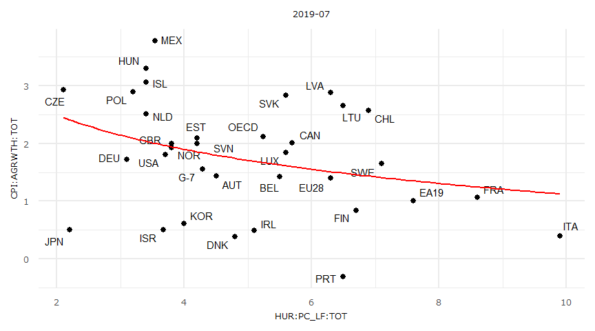
正規線形モデル
- 但し失業率はマイナス値を取らないため外挿は出来ない。
lmresult <- lm(y ~ x)
summary(lmresult)
Call:
lm(formula = y ~ x)

Residuals:
     Min       1Q   Median       3Q      Max
-1.80027 -0.41715 -0.00791  0.58511  1.74715

Coefficients:
            Estimate Std. Error t value   Pr(>|t|)
(Intercept)  2.69029    0.48715   5.522 0.00000434 ***
x           -0.18546    0.09165  -2.024     0.0514 .
---
Signif. codes:  0 '***' 0.001 '**' 0.01 '*' 0.05 '.' 0.1 ' ' 1

Residual standard error: 0.9451 on 32 degrees of freedom
Multiple R-squared:  0.1134,    Adjusted R-squared:  0.08574
F-statistic: 4.095 on 1 and 32 DF,  p-value: 0.05143
cor.test(x = x, y = y, alternative = "two")
    Pearson's product-moment correlation

data:  x and y
t = -2.0236, df = 32, p-value = 0.05143
alternative hypothesis: true correlation is not equal to 0
95 percent confidence interval:
 -0.605962887  0.001523003
sample estimates:
       cor
-0.3368162
dwtest(formula = y ~ x, alternative = "greater")
Durbin-Watson test
data: y ~ x
DW = 1.969, p-value = 0.4727
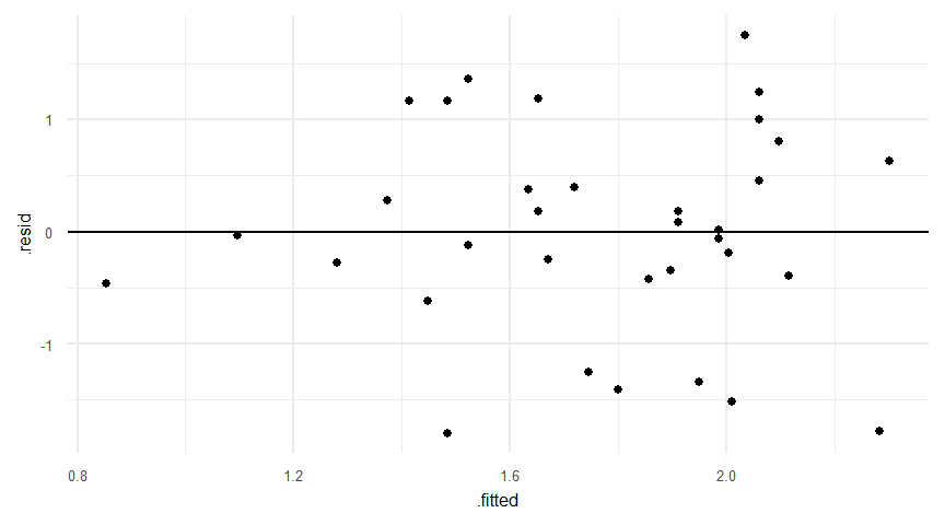
alternative hypothesis: true autocorrelation is greater than 0bptest(lmresult)
    studentized Breusch-Pagan test

data:  lmresult
BP = 1.1427, df = 1, p-value = 0.2851
ks.test(x = lmresult$residuals, y = "pnorm", mean = 0, sd = sd(lmresult$residuals), exact = T)
    One-sample Kolmogorov-Smirnov test

data:  lmresult$residuals
D = 0.10288, p-value = 0.8287
alternative hypothesis: two-sided
augment(lmresult)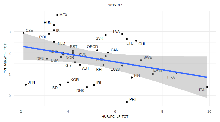
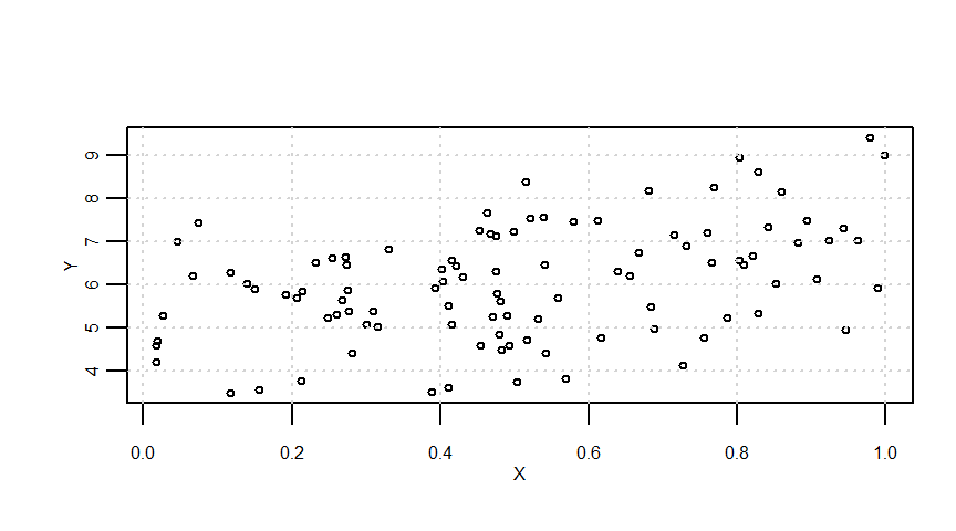
一般化最小二乗法
- 参照引用Webページ
一般化最小二乗法の例
# sample data
n <- 10^2
a <- 5
b <- 2
X <- runif(n = n)
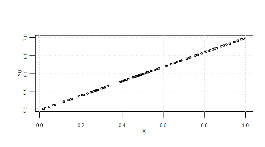
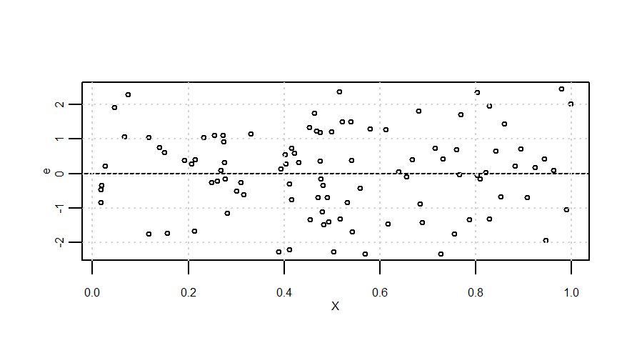
Y0 <- a + b * X
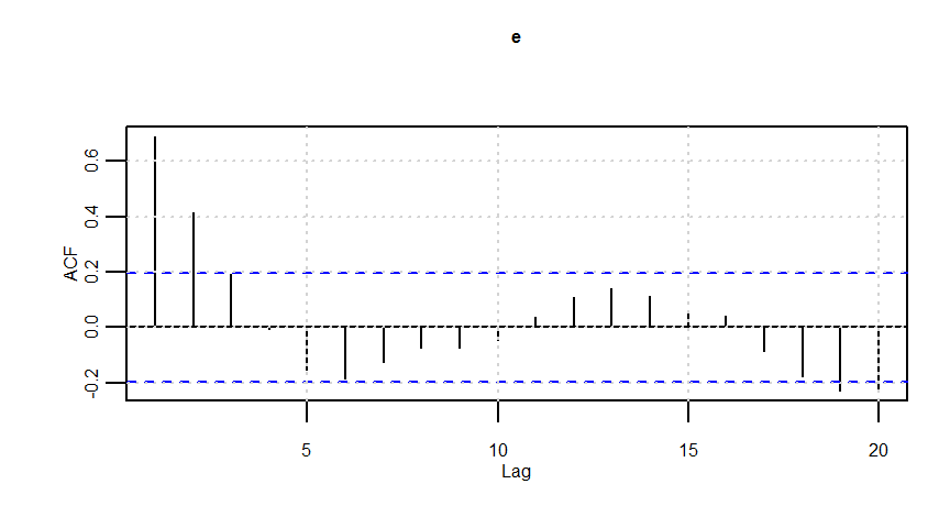
e <- arima.sim(model = list(order = c(1, 0, 0), ar = 0.8), n = n)
Y <- Y0 + e
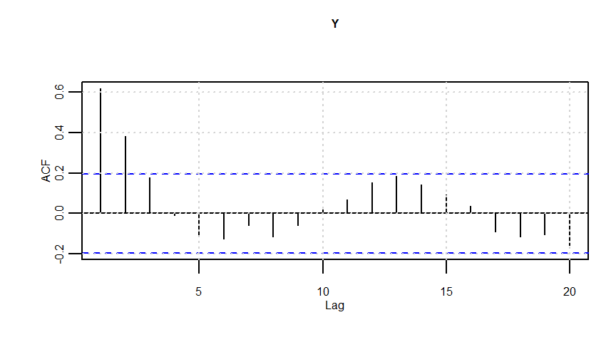
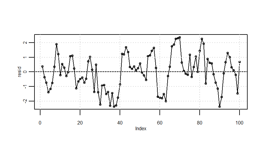
lmresult <- lm(Y ~ X)
resid <- lmresult$residualssummary(Y0) Min. 1st Qu. Median Mean 3rd Qu. Max.
5.035 5.561 5.963 6.009 6.455 6.995 summary(e) Min. 1st Qu. Median Mean 3rd Qu. Max.
-2.32888 -0.76964 0.12073 0.04418 0.94571 2.45313 summary(Y) Min. 1st Qu. Median Mean 3rd Qu. Max.
3.485 5.181 6.061 6.053 7.008 9.411 summary(lmresult)
Call:
lm(formula = Y ~ X)
Residuals:
Min 1Q Median 3Q Max
-2.37840 -0.80069 0.08605 0.91835 2.37592
Coefficients:
Estimate Std. Error t value Pr(>|t|)
(Intercept) 5.0091 0.2598 19.278 < 0.0000000000000002 ***
X 2.0696 0.4564 4.535 0.0000163 ***
---
Signif. codes: 0 '***' 0.001 '**' 0.01 '*' 0.05 '.' 0.1 ' ' 1
Residual standard error: 1.204 on 98 degrees of freedom
Multiple R-squared: 0.1735, Adjusted R-squared: 0.165
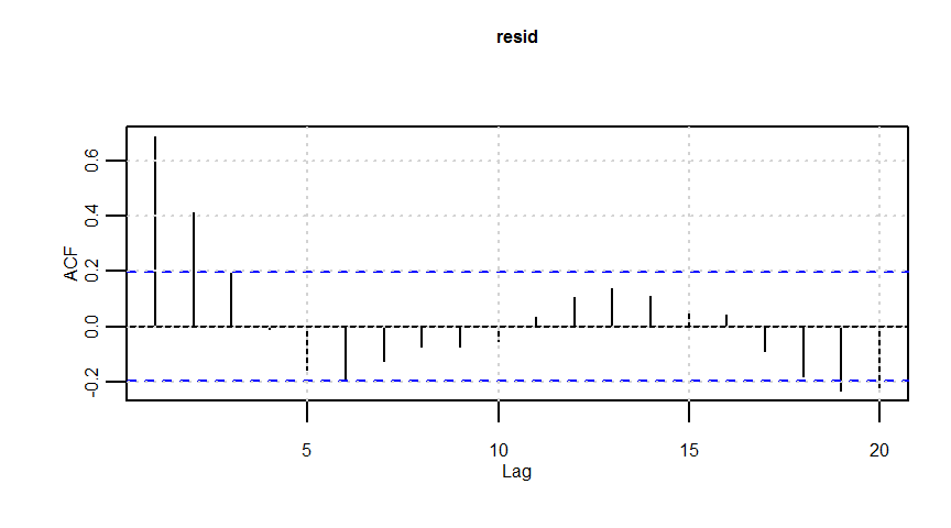
F-statistic: 20.57 on 1 and 98 DF, p-value: 0.00001633dwtest(lmresult)
    Durbin-Watson test

data:  lmresult
DW = 0.62201, p-value = 0.000000000001838
alternative hypothesis: true autocorrelation is greater than 0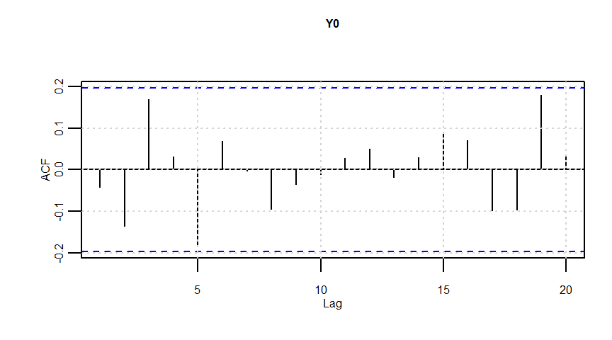
# gls
gls <- list()
gls[[1]] <- gls(model = Y ~ X, correlation = NULL)
gls[[2]] <- gls(model = Y ~ X, correlation = corARMA(p = 1))
gls[[3]] <- gls(model = Y ~ X, correlation = corARMA(p = 2))
aicmin <- which.min(sapply(gls, function(x) AIC(x)))aicmin[1] 2summary(gls[[aicmin]])Generalized least squares fit by REML
Model: Y ~ X
Data: NULL
AIC BIC logLik
263.5638 273.9036 -127.7819
Correlation Structure: AR(1)
Formula: ~1
Parameter estimate(s):
Phi
0.7039006
Coefficients:
Value Std.Error t-value p-value
(Intercept) 5.186552 0.3148668 16.472206 0
X 1.761248 0.2642722 6.664521 0
Correlation:
(Intr)
X -0.416
Standardized residuals:
Min Q1 Med Q3 Max
-1.94801599 -0.69554103 0.03924871 0.66888848 2.04689346
Residual standard error: 1.221517
Degrees of freedom: 100 total; 98 residual結果
gls <- list()
gls[[1]] <- gls(model = y ~ x, correlation = NULL)
gls[[2]] <- gls(model = y ~ x, correlation = corARMA(p = 1))
gls[[3]] <- gls(model = y ~ x, correlation = corARMA(p = 2))
aicmin <- which.min(sapply(gls, function(x) AIC(x)))aicmin[1] 1summary(gls[[aicmin]])Generalized least squares fit by REML
Model: y ~ x
Data: NULL
AIC BIC logLik
101.3925 105.7898 -47.69627
Coefficients:
Value Std.Error t-value p-value
(Intercept) 2.6902939 0.4871524 5.522489 0.0000
x -0.1854599 0.0916505 -2.023555 0.0514
Correlation:
(Intr)
x -0.943
Standardized residuals:
Min Q1 Med Q3 Max
-1.904811916 -0.441374863 -0.008368971 0.619082265 1.848601341
Residual standard error: 0.9451176
Degrees of freedom: 34 total; 32 residual線形回帰における回帰係数の信頼区間、母回帰式の区間推定、目的変数の予測区間、回帰直線の同時信頼区間
- 参考引用Webページ
- http://sphweb.bumc.bu.edu/otlt/MPH-Modules/BS/BS704_Confidence_Intervals/BS704_Confidence_Intervals_print.html
- http://lbm.ab.a.u-tokyo.ac.jp/~omori/kokusai11/kokusai11_1212.html
- http://www2.econ.osaka-u.ac.jp/~tanizaki/class/2016/basic_econome/03.pdf
- http://www.hil.hiroshima-u.ac.jp/sys2/a/kaikibunseki.pdf
- http://stat.sys.i.kyoto-u.ac.jp/titech/class/doc/lec20021114-9.pdf
- https://www.jstage.jst.go.jp/article/jscswabun/14/1/14_KJ00001896557/_pdf
- https://www2.isye.gatech.edu/~yxie77/isye2028/lecture12.pdf
\[y=\alpha x+\beta \]
回帰係数\(\alpha\)と\(\beta\)の推定
n <- length(x)  # サンプルサイズ
significant_level <- 0.05  # 有意水準
t_value <- qt(1 - significant_level/2, n - 2)  # 自由度n-2、有意水準0.05のt値
Sxx <- sum((x - mean(x))^2)  # 説明変数xの偏差平方和
Sxy <- sum((x - mean(x)) * (y - mean(y)))  # 説明変数xと目的変数yの積和
a <- Sxy/Sxx  # 回帰直線の傾きの推定量
b <- mean(y) - mean(x) * a  # 回帰直線の切片の推定量
estimated_y <- a * x + b  # 推定されたy
residuals <- y - estimated_y  # 残差
sigma <- sqrt(sum((residuals - mean(residuals))^2)/(n - 2))  # 残差標準偏差
a
b
lmresult$coefficients[1] -0.1854599
[1] 2.690294
(Intercept) X
5.009075 2.069591 回帰係数\(\alpha\)と\(\beta\)それぞれの信頼区間
\[\hat{\alpha}\pm t_{(n-2,\frac{0.05}{2})}\times\frac{\hat{\sigma}}{\sqrt{S_{xx}}}\quad,\quad \hat{\beta}\pm t_{(n-2,\frac{0.05}{2})}\times\hat{\sigma}\times{\sqrt{\frac{1}{n}+\frac{\bar{x}^{2}}{S_{xx}}}}\]
ci <- t_value * sigma/sqrt(Sxx)
a - ci
a + ci
ci <- t_value * sigma * sqrt(1/n + mean(x)^2/Sxx)
b - ci
b + ci
# confint {stats}で直接求められます
confint(lmresult, level = 0.95)
[1] -0.3721458
[1] 0.001226093
[1] 1.697997
[1] 3.682591
2.5 % 97.5 %
(Intercept) 4.493456 5.524693
X 1.163944 2.975237真の回帰式(母回帰式)の存在範囲推定=母回帰式の区間推定
- なおggplotでse = Tとした場合に表示される信頼区間はこの母回帰式の区間推定になります。
\[(\hat{\alpha}x_{0}+\hat{\beta})\pm t_{(n-2,\frac{0.05}{2})}\times\sqrt{\frac{1}{n}+\frac{(x-\bar{x})^{2}}{S_{xx}}}\times \hat{\sigma}\]
ci <- t_value * sqrt(1/n + ((x - mean(x))^2)/Sxx) * sigma
lower1 <- estimated_y - ci
upper1 <- estimated_y + ci
par(mar = c(2.5, 2.5, 0.5, 0.5), mgp = c(1, 0.5, 0), cex.lab = 0.8, cex.axis = 0.8, cex = 0.5)
plot(x, y, ylim = c(min(y, lower1, upper1), max(y, lower1, upper1)))
lines(x, estimated_y)
cidf <- data.frame(x, upper1, lower1)
cidf <- cidf[order(cidf$x), ]
lines(x = cidf$x, y = cidf$upper1, col = "red", type = "l")
lines(x = cidf$x, y = cidf$lower1, col = "red", type = "l")
grid()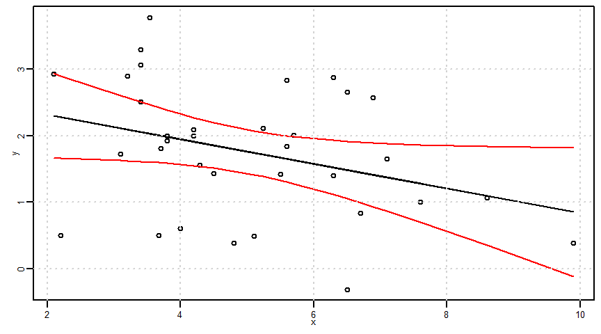
説明変数\(x\)の値を\(x_{0}\)に指定したときの目的変数\(y\)の信頼区間=予測区間
\[(\hat{\alpha}x_{0}+\hat{\beta})\pm t_{(n-2,\frac{0.05}{2})}\times\sqrt{1+\frac{1}{n}+\frac{(x-\bar{x})^{2}}{S_{xx}}}\times \hat{\sigma}\]
ci <- t_value * sqrt(1 + 1/n + ((x - mean(x))^2)/Sxx) * sigma
lower2 <- estimated_y - ci
upper2 <- estimated_y + ci
par(mar = c(2.5, 2.5, 0.5, 0.5), mgp = c(1, 0.5, 0), cex.lab = 0.8, cex.axis = 0.8, cex = 0.5)
plot(x, y, ylim = c(min(y, lower2, upper2), max(y, lower2, upper2)))
lines(x, estimated_y)
cidf <- data.frame(x, upper2, lower2)
cidf <- cidf[order(cidf$x), ]
lines(x = cidf$x, y = cidf$upper2, col = "red", type = "l")
lines(x = cidf$x, y = cidf$lower2, col = "red", type = "l")
grid()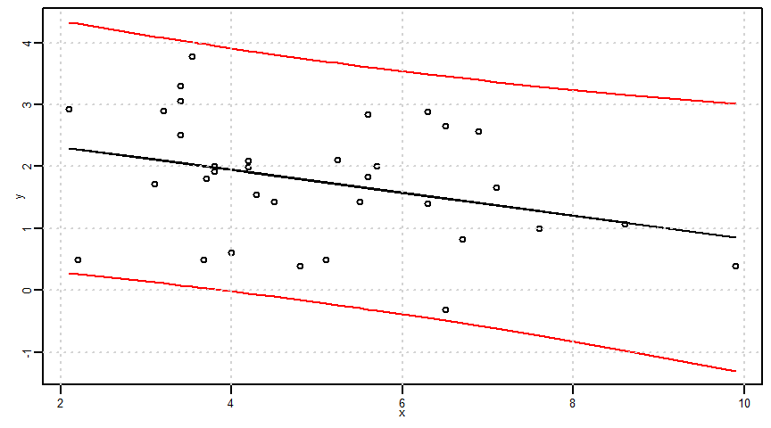
\(x=x_{0}\)だけでなく、すべての\(x\)に対する回帰直線の同時信頼区間
\[(\hat{\alpha}x_{0}+\hat{\beta})\pm \sqrt{2F_{(2,n-2,\frac{0.05}{2})}}\times\sqrt{\frac{1}{n}+\frac{(x-\bar{x})^{2}}{S_{xx}}}\times \hat{\sigma}\]
ci <- sqrt(2 * qf(significant_level, 2, n - 2)) * sqrt(1/n + ((x - mean(x))^2)/Sxx) * sigma
lower3 <- estimated_y - ci
upper3 <- estimated_y + ci
par(mar = c(2.5, 2.5, 0.5, 0.5), mgp = c(1, 0.5, 0), cex.lab = 0.8, cex.axis = 0.8, cex = 0.5)
plot(x, y, ylim = c(min(y, lower3, upper3), max(y, lower3, upper3)))
lines(x, estimated_y)
cidf <- data.frame(x, upper3, lower3)
cidf <- cidf[order(cidf$x), ]
lines(x = cidf$x, y = cidf$upper3, col = "red", type = "l")
lines(x = cidf$x, y = cidf$lower3, col = "red", type = "l")
grid()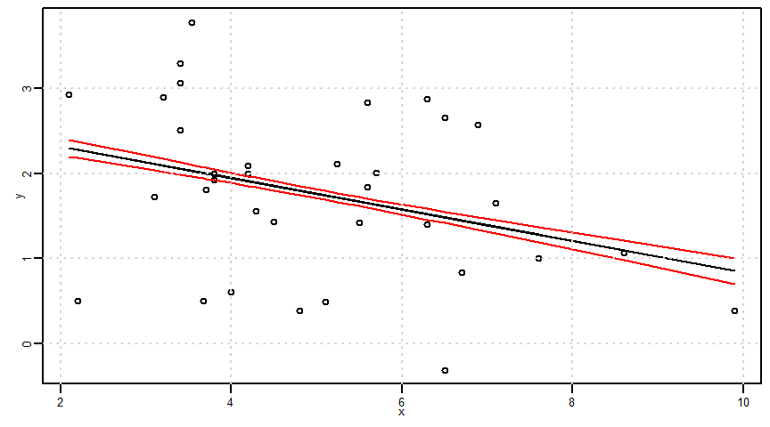
ベイズ推定:単回帰、説明変数:連続量、応答変数:連続量 + 誤差構造:正規分布
- 参照引用Webページ
- https://github.com/MatsuuraKentaro/RStanBook
- https://stan-ja.github.io/gh-pages-html/
- http://statmodeling.hatenablog.com/archive/category/Stan
- http://statmodeling.hatenablog.com/archive/category/R
- https://logics-of-blue.com/stan%e3%81%ab%e3%82%88%e3%82%8b%e3%83%99%e3%82%a4%e3%82%ba%e6%8e%a8%e5%ae%9a%e3%81%ae%e5%9f%ba%e7%a4%8e/
- https://logics-of-blue.com/%e3%83%99%e3%82%a4%e3%82%ba%e3%81%a8mcmc%e3%81%a8%e7%b5%b1%e8%a8%88%e3%83%a2%e3%83%87%e3%83%ab%e3%81%ae%e9%96%a2%e4%bf%82/
- https://heavywatal.github.io/rstats/stan.html
\[y:確率変数,\quad p(y):確率分布,\quad y\sim p(y),\quad \theta:パラメータ,\quad Y:観測値,\quad p(\theta|Y):事後分布,\quad p(\theta):事前分布,\quad p(Y|\theta):尤度 \]
\[p(\theta|Y)=\frac{p(Y|\theta)p(\theta)}{p(Y)}\propto p(y|\theta)p(\theta)\]
\[p(y|Y):予測分布,\quad p(y|Y)= \int p(y|\theta) p(\theta|Y)d\theta,\quad \int p(y|\theta) p(\theta) d\theta:事前予測分布\]
\[ Y[n]=b+aX[n]+\epsilon[n],\quad \epsilon[n]\sim {\rm N}(0,\sigma),\quad Y[n]\sim {\rm N}(b+aX[n],\sigma) \]
# 並列化。忘れると時間がかかって大変なことになる(*但し進捗を見たい場合は並列化なしで実行)。
library(rstan)
rstan_options(auto_write = T)
options(mc.cores = parallel::detectCores())
data <- list(N = nrow(dataf), x = x, y = y)# モデルの作成
model01 <- "
data {
int N;
real x[N];
real y[N];
}
parameters {
real a;
real b;
real<lower=0> sigma;
}
model {
for(n in 1:N) {
y[n] ~ normal(b+a*x[n],sigma);
}
}
"# ベイズ推定の結果
fit <- stan(model_code = model01, data = data, iter = 1400, warmup = 400, thin = 1, chains = 3)
fit
# lp__:対数確率密度Inference for Stan model: f94c8d0515da3c11dd96e78e1fff8216.
3 chains, each with iter=1400; warmup=400; thin=1;
post-warmup draws per chain=1000, total post-warmup draws=3000.
mean se_mean sd 2.5% 25% 50% 75% 97.5% n_eff Rhat
a -0.19 0.00 0.10 -0.37 -0.25 -0.19 -0.12 0.01 1173 1
b 2.69 0.01 0.51 1.68 2.35 2.69 3.03 3.69 1157 1
sigma 0.98 0.00 0.12 0.77 0.90 0.97 1.06 1.25 1459 1
lp__ -15.66 0.04 1.22 -18.76 -16.26 -15.34 -14.75 -14.23 853 1
Samples were drawn using NUTS(diag_e) at Wed Dec 04 07:35:37 2019.
For each parameter, n_eff is a crude measure of effective sample size,
and Rhat is the potential scale reduction factor on split chains (at
convergence, Rhat=1).get_inits(fit)[[1]]
[[1]]$a
[1] -1.717434
[[1]]$b
[1] 0.03078339
[[1]]$sigma
[1] 0.2950896
[[2]]
[[2]]$a
[1] 0.1754775
[[2]]$b
[1] -1.308109
[[2]]$sigma
[1] 1.056373
[[3]]
[[3]]$a
[1] -1.35683
[[3]]$b
[1] -1.782972
[[3]]$sigma
[1] 6.41184get_seed(fit)[1] 272825193traceplot(fit) + theme(axis.text = element_text(size = 5), strip.text = element_text(size = 5), legend.text = element_text(size = 5), legend.title = element_text(size = 5))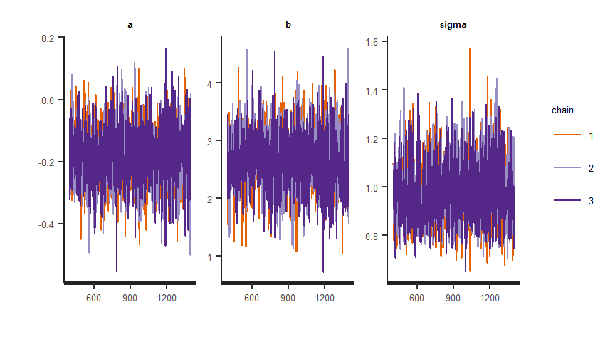
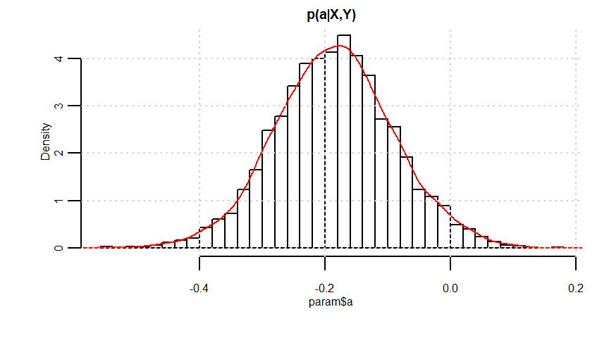
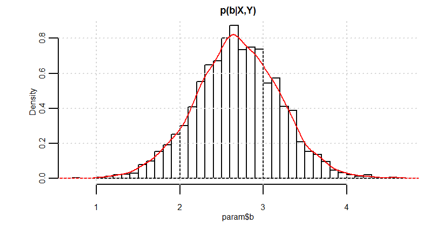
param <- rstan::extract(fit)
quantile(param$a, probs = c(0.025, 0.975))
quantile(param$b, probs = c(0.025, 0.975))
quantile(param$sigma, probs = c(0.025, 0.975))
2.5% 97.5%
-0.374109213 0.008218902
2.5% 97.5%
1.676596 3.688038
2.5% 97.5%
0.7670327 1.2503353 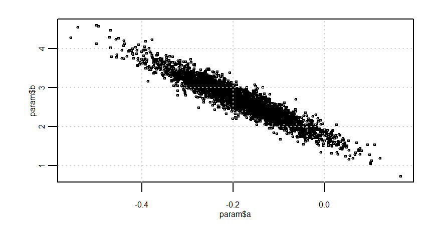
# 予測分布
x <- 3
y <- param$b + param$a * x
y_pred <- rnorm(n = length(param$a), mean = y, sd = param$sigma)
mcmc_df <- data.frame(a = param$a, b = param$b, sigma = param$sigma, y_pred, y)
apply(mcmc_df, 2, function(x) quantile(x, probs = c(0.025, 0.975)))
a b sigma y_pred y
2.5% -0.374109213 1.676596 0.7670327 0.08879189 1.631504
97.5% 0.008218902 3.688038 1.2503353 4.25269108 2.644482金融時系列データのクラスタリング
- 参照引用Webページ
- 非類似度分類アルゴリズム(quoted from https://www.rdocumentation.org/packages/TSclust/versions/1.2.4/topics/diss )
- “ACF” Autocorrelation-based method. diss.ACF.
- “AR.LPC.CEPS” Linear Predictive Coding ARIMA method. This method has two value-per-series arguments, the ARIMA order, and the seasonality. diss.AR.LPC.CEPS.
- “AR.MAH” Model-based ARMA method. diss.AR.MAH.
- “AR.PIC” Model-based ARMA method. This method has a value-per-series argument, the ARIMA order. diss.AR.PIC.
- “CDM” Compression-based dissimilarity method. diss.CDM.
- “CID” Complexity-Invariant distance. diss.CID.
- “COR” Correlation-based method. diss.COR.
- “CORT” Temporal Correlation and Raw values method. diss.CORT.
- “DTWARP” Dynamic Time Warping method. diss.DTWARP.
- “DWT” Discrete wavelet transform method. diss.DWT.
- “EUCL” Euclidean distance. diss.EUCL. For many more convetional distances, see link[stats]{dist}, though you may need to transpose the dataset.
- “FRECHET” Frechet distance. diss.FRECHET.
- “INT.PER” Integrate Periodogram-based method. diss.INT.PER.
- “NCD” Normalized Compression Distance. diss.NCD.
- “PACF” Partial Autocorrelation-based method. diss.PACF.
- “PDC” Permutation distribution divergence. Uses the pdc package. pdcDist for additional arguments and details. Note that series given by numeric matrices are interpreted row-wise and not column-wise, opposite as in pdcDist.
- “PER” Periodogram-based method. diss.PER.
- “PRED” Prediction Density-based method. This method has two value-per-series agument, the logarithm and difference transform. diss.PRED.
- “MINDIST.SAX” Distance that lower bounds the Euclidean, based on the Symbolic Aggregate approXimation measure. diss.MINDIST.SAX.
- “SPEC.LLR” Spectral Density by Local-Linear Estimation method. diss.SPEC.LLR.
- “SPEC.GLK” Log-Spectra Generalized Likelihood Ratio test method. diss.SPEC.GLK.
- “SPEC.ISD” Intregated Squared Differences between Log-Spectras method. diss.SPEC.ISD.
head(tsdata)
tail(tsdata)
k <- 3  # number of group.bond,fx,stockindex
n <- 2  # two series each
Date T10Y2Y T10Y3M DEXUSEU DEXJPUS SP500 NIKKEI225
812 2016-12-01 1.295238 1.980000 1.054462 115.9981 2246.629 19066.03
813 2017-01-01 1.226000 1.913500 1.063495 114.8721 2275.116 19194.06
814 2017-02-01 1.217895 1.892632 1.065021 112.9116 2329.911 19188.73
815 2017-03-01 1.168696 1.733913 1.069104 112.9165 2366.822 19340.18
816 2017-04-01 1.056316 1.488947 1.071380 110.0910 2359.309 18736.39
817 2017-05-01 1.001818 1.400455 1.104986 112.2436 2395.346 19726.76
Date T10Y2Y T10Y3M DEXUSEU DEXJPUS SP500 NIKKEI225
842 2019-06-01 0.2600000 -0.14550000 1.129515 108.0685 2890.166 21060.21
843 2019-07-01 0.2240909 -0.08590909 1.121145 108.2864 2996.114 21593.68
844 2019-08-01 0.0550000 -0.36409091 1.112868 106.1886 2897.498 20629.68
845 2019-09-01 0.0515000 -0.23500000 1.101120 107.5400 2982.156 21585.46
846 2019-10-01 0.1554545 0.02818182 1.105818 108.1368 2977.675 22197.47
847 2019-11-01 0.1994737 0.24000000 1.105058 108.8579 3104.905 23278.09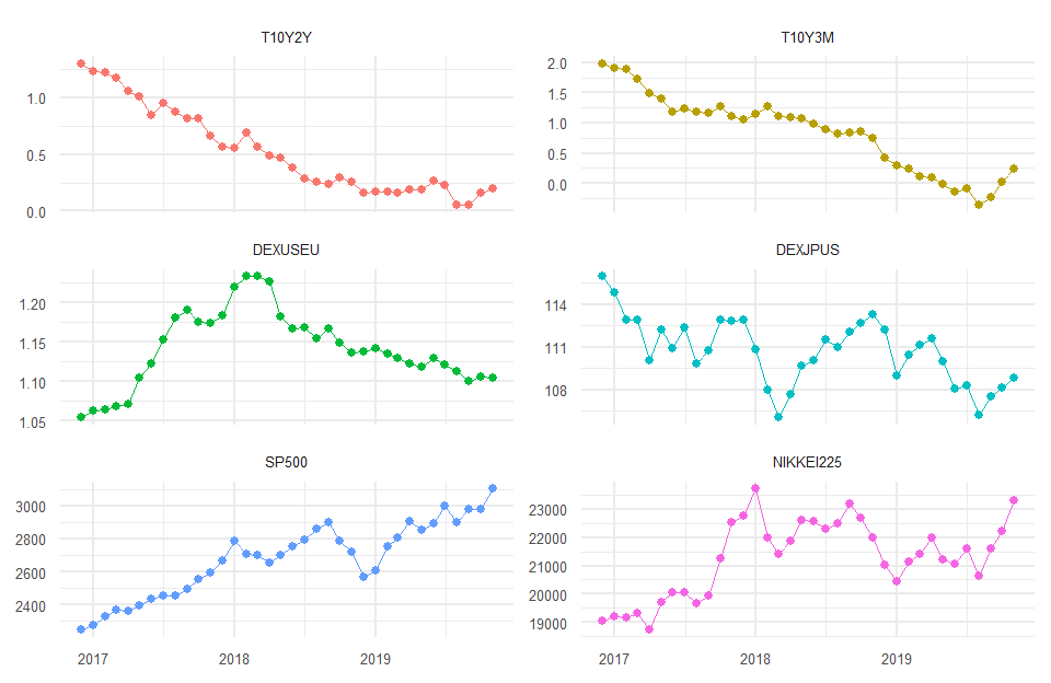
library(TSclust)
library(dendextend)
METHODs <- c("ACF", "AR.LPC.CEPS", "AR.MAH", "AR.PIC", "CDM", "CID", "COR", "CORT", "DTWARP", "DWT", "EUCL", "FRECHET", "INT.PER", "NCD", "PACF", "PDC", "PER", "PRED", "MINDIST.SAX", "SPEC.LLR", "SPEC.GLK", "SPEC.ISD")
cluster_eval <- data.frame()
hclust_method <- "complete"
cnt <- 1
dendrogramData <- list()
for (mmm in seq(METHODs)) {
    diss_method <- METHODs[mmm]
    tryCatch({
        d <- diss(SERIES = tsdata[, -1], METHOD = diss_method)
        h <- hclust(d = d, method = hclust_method)
        cluster_eval[cnt, 1] <- diss_method
        cluster_eval[cnt, 2] <- cluster.evaluation(rep(seq(k), rep(n, k)), as.factor(cutree(tree = h, k = k)))
        cluster_eval[cnt, 3] <- hclust_method
        dendrogramData[[cnt]] <- as.dendrogram(h)
        cnt <- cnt + 1
    }, error = function(e) {
    })
}
colnames(cluster_eval) <- c("Dissimilarity measure method", "Evaluation", "Hierarchical clustering agglomeration method")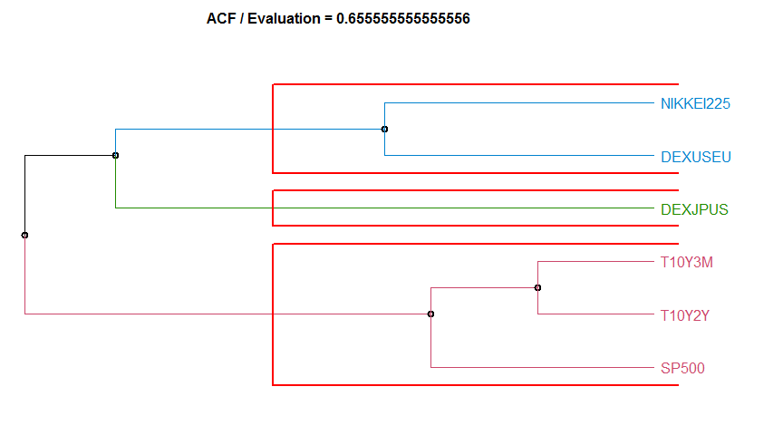
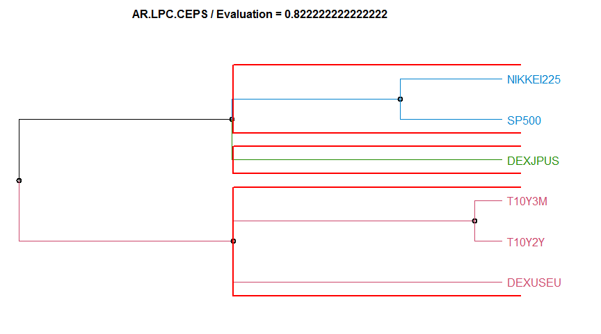
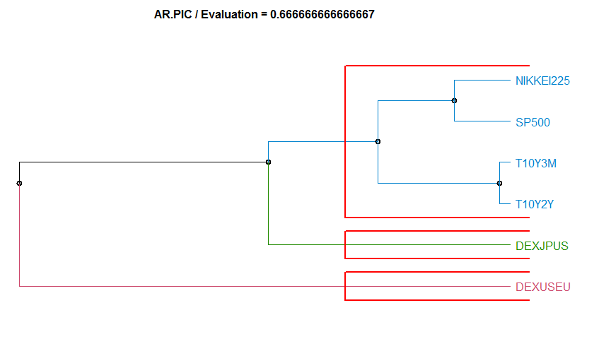
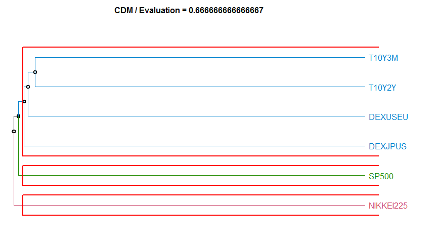
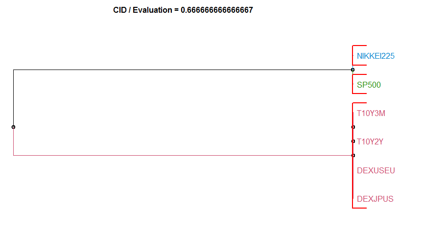
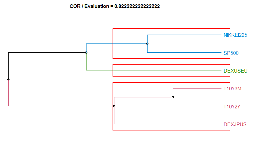

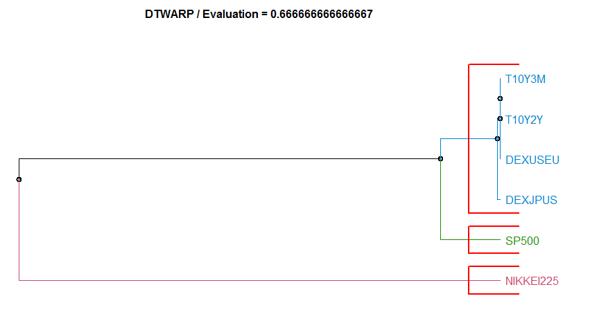
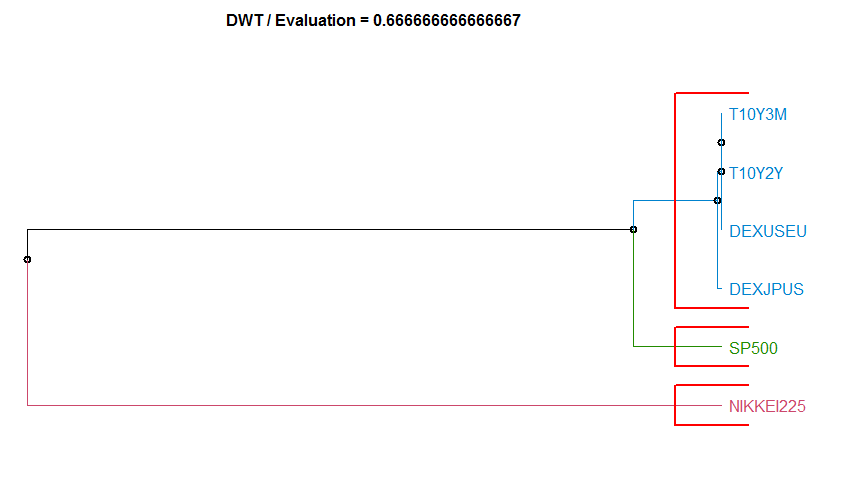


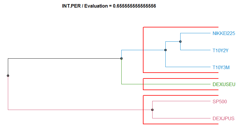
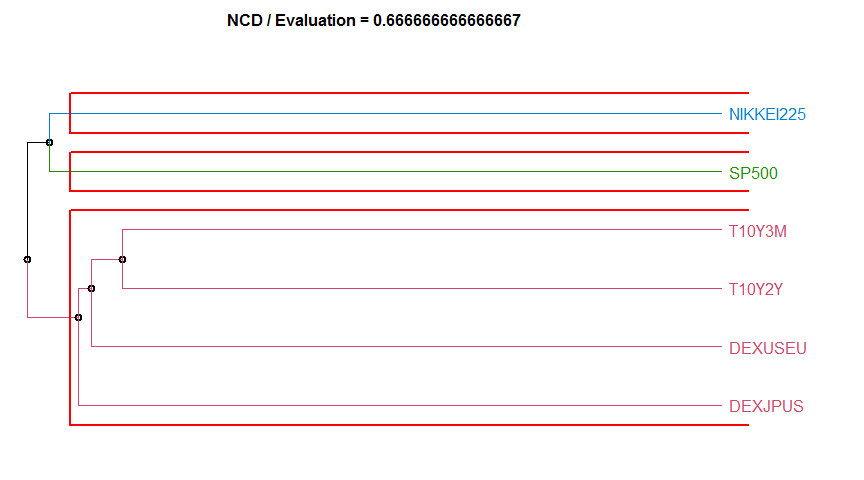
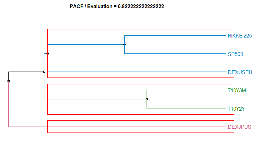
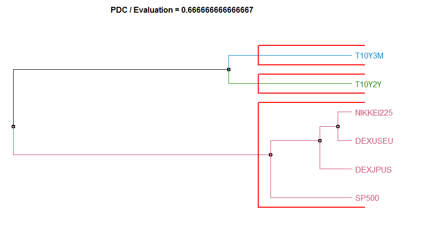
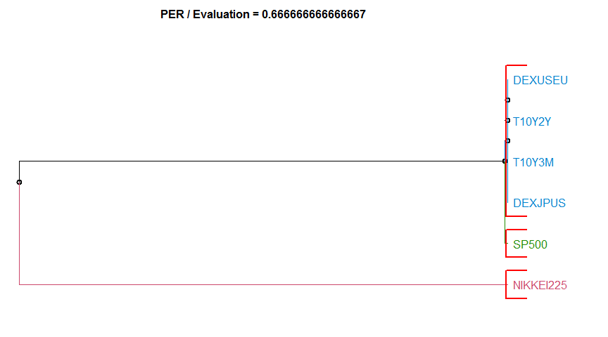

   Dissimilarity measure method Evaluation Hierarchical clustering agglomeration method
1                           ACF  0.6555556                                     complete
2                   AR.LPC.CEPS  0.8222222                                     complete
3                        AR.PIC  0.6666667                                     complete
4                           CDM  0.6666667                                     complete
5                           CID  0.6666667                                     complete
6                           COR  0.8222222                                     complete
7                          CORT  0.6666667                                     complete
8                        DTWARP  0.6666667                                     complete
9                           DWT  0.6666667                                     complete
10                         EUCL  0.6666667                                     complete
11                      FRECHET  0.6666667                                     complete
12                      INT.PER  0.6555556                                     complete
13                          NCD  0.6666667                                     complete
14                         PACF  0.8222222                                     complete
15                          PDC  0.6666667                                     complete
16                          PER  0.6666667                                     complete
17                     SPEC.LLR  0.8222222                                     complete
18                     SPEC.GLK  0.8222222                                     complete
19                     SPEC.ISD  0.8222222                                     complete
オバマ政権とトランプ政権でNASDAQ指数の前営業日比騰落回数に差はあるか否か
- オバマ政権とトランプ政権でNASDAQ指数の前営業日比騰落回数に差はあるか否か(独立性の検定)
- The Obama administration:2009-01-20 - 2017-01-19,2922 days
- The Trump administration:2017-01-20 ~ 2019-12-02,1047 days
- Source:FRED,NASDAQ OMX Group
\[\chi^2統計量=\sum_{i=1}^2 \sum_{j=1}^2 \frac{(O_{ij}-E_{ij})^2}{E_{ij}}\]
| Up | Down | Total | |
|---|---|---|---|
| Obama | 1,120 | 895 | 2,015 |
| Trump | 411 | 311 | 722 |
| Total | 1,531 | 1,206 | 2,737 |
| Up | Down | Total | |
|---|---|---|---|
| Obama | 1,127 | 888 | 2,015 |
| Trump | 404 | 318 | 722 |
| Total | 1,531 | 1,206 | 2,737 |
obs_data POTUS Change frequency
1 Obama Up 1120
2 Obama Down 895
3 Trump Up 411
4 Trump Down 311cross_data <- xtabs(frequency ~ ., obs_data)
cross_data Change
POTUS Down Up
Obama 895 1120
Trump 311 411# H0:オバマ政権とトランプ政権でNASDAQ指数の前営業日比騰落回数に差は見られない。
chisq.test(cross_data, correct = F)
    Pearson's Chi-squared test

data:  cross_data
X-squared = 0.38844, df = 1, p-value = 0.5331